Krugmanwellscanadianmicro2

Price Elasticity of Demand

Let’s return to our example from Appendix 3A, the demand for maple syrup, to look at the algebra of elasticity. There, we started with a very simple linear demand curve in its simplest form:

where P denotes the price (in dollars per litre), Q^d denotes the quantity (in millions of litres), and a and b are positive constants.

If we isolate Q^d as a function of the other terms, we get:

According to this equation, if the price of maple syrup increases by $1 per litre (i.e., ΔP = 1), then the quantity of maple syrup demanded decreases by . Therefore, the ratio is equal to , a fact we will need to use later.

Now we can look more closely at the price elasticity of demand, which was expressed in Equation 6-5 as:

This equation can be simplified after rewriting it using algebraic terms such as ΔQ^d for the change in Q^d = Q₂ – Q₁, ΔP for the change in P = P₂ – P₁, and using the values P and Q^d instead of the midpoint values:

When interpreting the price elasticity of demand, we only look at the absolute value, so we can redefine the price elasticity of demand, E_d, as:

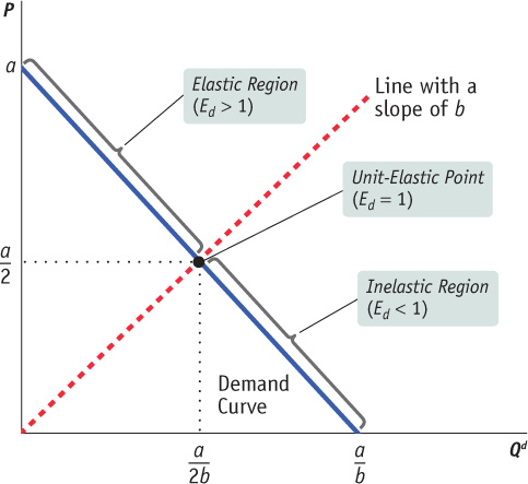
This formula for the price elasticity of demand comes in handy when analyzing a graph of the demand curve. As we move along the demand curve in Figure 6A-1, b remains constant but the ratio of P divided by Q^d varies. Therefore the price elasticity of demand varies as we move along a linear demand curve. The ratio P/Q^d is the slope of the line passing through the origin and the point (Q^d, P) on the demand curve (because the rise of the line is P and the run is Q^d). When the slope of the line is equal to b, the point at which this line intersects the demand curve has a price elasticity of demand of one—the unit-elastic point. All lines steeper than this one intersect at points on the demand curve with a price elasticity of demand greater than one—the region of elastic demand points. Similarly, the points on the demand curve that lie below the unit-elastic point have price elasticity of demand less than one—the inelastic points.

Figure6A-1Price Elasticity along a Linear Demand Curve Price elasticity varies along the demand curve. A line with a slope b that passes through the origin will intersect the demand curve. At the point of intersection, price elasticity is 1 (the unit-elastic point). To the left of the point, price elasticity is greater than 1. To the right, price elasticity is less than 1.

These regions can be determined algebraically by first substituting P = a – b × Q^d into Equation 6A-2 to express E_d in terms of a, b, and Q^d:

Notice that by carefully selecting values of Q^d, we can generate values of E_d that are less than, greater than, or equal to 1.