19.4 The Supply of Labour
Up to this point we have focused on the demand for factors, which determines the quantities demanded of labour, capital, or land by producers as a function of their factor prices. What about the supply of factors?
In this section we focus exclusively on the supply of labour. We do this for two reasons. First, in the modern Canadian economy, labour is the most important factor of production, accounting for most of factor income. Second, as we’ll see,labour supply is the area in which factor markets look most different from markets for goods and services.
Work versus Leisure
In the labour market, the roles of firms and households are the reverse of what they are in markets for goods and services. A good such as wheat is supplied by firms and demanded by households; labour, though, is demanded by firms and supplied by households. How do people decide how much labour to supply?
As a practical matter, most people have limited control over their work hours: either you take a job that involves working a set number of hours per week, or you don’t get the job at all. To understand the logic of labour supply, however, it helps to put realism to one side for a bit and imagine an individual who can choose to work as many or as few hours as he or she likes.
Decisions about labour supply result from decisions about utility-
Why wouldn’t such an individual work as many hours as possible? Because workers are human beings, too, and have other uses for their time. An hour spent on the job is an hour not spent on other, presumably more pleasant, activities. So the decision about how much labour to supply involves making a decision about utility-
Leisure is time available for purposes other than earning money to buy marketed goods.
By working, people earn income that they can use to buy goods. The more hours an individual works, the more goods he or she can afford to buy. But this increased purchasing power comes at the expense of a reduction in leisure, the time spent not working. (Leisure doesn’t necessarily mean time spent goofing off. It could mean time spent with one’s family, pursuing hobbies, exercising, and so on.) And though purchased goods yield utility, so does leisure. Indeed, we can think of leisure itself as a normal good, which most people would like to consume more of as their incomes increase.
How does a rational individual decide how much leisure to consume? By making a marginal comparison, of course. In analyzing consumer choice, we asked how a utility-
Consider Clive, an individual who likes both leisure and the goods money can buy. Suppose that his wage rate is $10 per hour. In deciding how many hours he wants to work, he must compare the marginal utility of an additional hour of leisure with the additional utility he gets from $10 worth of goods. If $10 worth of goods adds more to his total utility than an additional hour of leisure, he can increase his total utility by giving up an hour of leisure in order to work an additional hour. If an extra hour of leisure adds more to his total utility than $10 worth of goods, he can increase his total utility by working one fewer hour in order to gain an hour of leisure.
At Clive’s optimal labour supply choice, then, his marginal utility of one hour of leisure is equal to the marginal utility he gets from the goods that his hourly wage can purchase. This is very similar to the optimal consumption rule we encountered in Chapter 10, except that it is a rule about time rather than money.
Our next step is to ask how Clive’s decision about time allocation is affected when his wage rate changes.
Wages and Labour Supply
Suppose that Clive’s wage rate doubles, from $10 to $20 per hour. How will he change his time allocation?
You could argue that Clive will work longer hours, because his incentive to work has increased: by giving up an hour of leisure, he can now gain twice as much money as before. But you could equally well argue that he will work less, because he doesn’t need to work as many hours to generate the income to pay for the goods he wants.
As these opposing arguments suggest, the quantity of labour Clive supplies can either rise or fall when his wage rate rises. To understand why, let’s recall the distinction between substitution effects and income effects that we learned in Chapter 10 and its appendix. We saw there that a price change affects consumer choice in two ways: by changing the opportunity cost of a good in terms of other goods (the substitution effect) and by making the consumer richer or poorer (the income effect).
Now think about how a rise in Clive’s wage rate affects his demand for leisure. The opportunity cost of leisure—
So in the case of labour supply, the substitution effect and the income effect work in opposite directions. If the substitution effect is so powerful that it dominates the income effect, an increase in Clive’s wage rate leads him to supply more hours of labour. If the income effect is so powerful that it dominates the substitution effect, an increase in the wage rate leads him to supply fewer hours of labour.
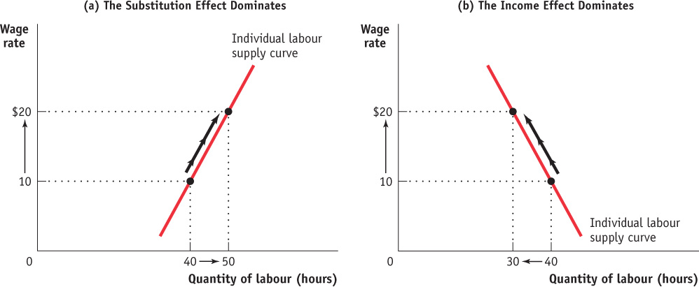
The individual labour supply curve shows how the quantity of labour supplied by an individual depends on that individual’s wage rate.
We see, then, that the individual labour supply curve—the relationship between the wage rate and the number of hours of labour supplied by an individual worker—
Figure 19-11 illustrates the two possibilities for labour supply. If the substitution effect dominates the income effect, the individual labour supply curve slopes upward; panel (a) shows an increase in the wage rate from $10 to $20 per hour leading to a rise in the number of hours worked from 40 to 50. However, if the income effect dominates, the quantity of labour supplied goes down when the wage rate increases. Panel (b) shows the same rise in the wage rate leading to a fall in the number of hours worked from 40 to 30. (Economists refer to an individual labour supply curve that contains both upward-
WHY YOU CAN’T FIND A CAB WHEN IT’S RAINING
Everyone says that you can’t find a taxi when you really need one—
The reason is that the hourly wage rate of a taxi driver depends on the weather: when it’s raining, drivers get more fares and therefore earn more per hour. But it seems that the income effect of this higher wage rate outweighs the substitution effect.
This behaviour leads the authors of the study to question drivers’ rationality. They point out that if taxi drivers thought in terms of the long run, they would realize that rainy days and nice days tend to average out and that their high earnings on a rainy day don’t really affect their long-
Is a negative response of the quantity of labour supplied to the wage rate a real possibility? Yes: many labour economists believe that income effects on the supply of labour may be somewhat stronger than substitution effects. The most compelling piece of evidence for this belief comes from Canadians’ increasing consumption of leisure over the past century. At the end of the nineteenth century, wages adjusted for inflation were only about one-
Shifts of the Labour Supply Curve
Now that we have examined how income and substitution effects shape the individual labour supply curve, we can turn to the market labour supply curve. In any labour market, the market supply curve is the horizontal sum of the individual labour supply curves of all workers in that market. A change in any factor other than the wage that alters workers’ willingness to supply labour causes a shift of the labour supply curve. A variety of factors can lead to such shifts, including changes in preferences and social norms, changes in population, changes in opportunities, and changes in wealth.
Changes in Preferences and Social Norms Changes in preferences and social norms can lead workers to increase or decrease their willingness to work at any given wage. A striking example of this phenomenon is the large increase in the number of employed women—particularly married employed women—that has occurred in Canada and the United States since the 1960s. Until that time, women who could afford to largely avoided working outside the home. Changes in preferences and norms in post–World War II North America (helped along by the invention of labour-saving home appliances such as washing machines, increasing urbanization of the population, and higher female education levels) have induced large numbers of North American women to join the workforce—a phenomenon often repeated in other countries that experience similar social and technological forces.
Changes in Population Changes in the population size generally lead to shifts of the labour supply curve. A larger population tends to shift the labour supply curve rightward as more workers are available at any given wage; a smaller population tends to shift the labour supply curve leftward. From 1987 to 2013, the Canadian labour force has grown approximately 1.3% per year, largely due to immigration. As a result, from 1987 to 2013 the Canadian labour market had a rightward-shifting labour supply curve. However, while the population continued to grow in the recession years 1992 and 2009, the growth rate of the labour force slowed as workers, disillusioned by bad job prospects, left the labour force. In fact, 1992 was the one year the Canadian labour supply curve did not shift right at all.
Changes in Opportunities At one time, teaching was the only occupation considered suitable for well-educated women. However, as opportunities in other professions opened up to women starting in the 1960s, many women left teaching and potential female teachers chose other careers. This generated a leftward shift of the supply curve for teachers, reflecting a fall in the willingness to work at any given wage and forcing school districts to pay more to maintain an adequate teaching staff. These events illustrate a general result: when superior alternatives arise for workers in another labour market, the supply curve in the original labour market shifts leftward as workers move to the new opportunities. Similarly, when opportunities diminish in one labour market—say, layoffs in the manufacturing industry due to increased foreign competition—the supply in alternative labour markets increases as workers move to these other markets.
THE OVERWORKED AMERICAN?
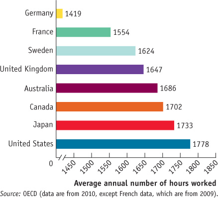
Americans today may work less than they did a hundred years ago, but they still work more than workers in any other industrialized country, including Canada.
This figure compares average annual hours worked in the United States with those worked in other industrialized countries. The differences result from a combination of Americans’ longer workweeks and shorter vacations. For example, the great majority of full-time American workers put in at least 40 hours per week. Until recently, however, a government mandate limited most French workers to a 35-hour workweek; collective bargaining has achieved a similar reduction in the workweek for many German workers.
In 2011, American workers got, on average, eight paid vacation days, but 23% of American workers got none at all. (Of developed nations, Canadian and Japanese workers are second worst off with a minimum of 10 paid vacation days per year.) In contrast, German workers are guaranteed six weeks of paid vacation a year. Also, American workers use fewer of the vacation days they are entitled to than do workers in other industrialized countries. A 2011 survey found that only 57% of American workers use all the vacation days they are entitled to, compared to 89% in France.
Why do Americans work so much more than others? Unlike their counterparts in other industrialized countries, Americans are not legally entitled to paid vacation days; as a result, the average American worker gets fewer of them. Moreover, anecdotal evidence suggests that during the recent recession, with its high rates of unemployment, American workers became more reluctant to use the vacation days they were entitled to.
Once again it is good to be a Canadian worker, but perhaps only as compared to Japanese and American workers.
Changes in Wealth A person whose wealth increases will buy more normal goods, including leisure. So when a class of workers experiences a general rise in their wealth levels—say, due to a stock market boom—the income effect from the wealth increase will shift the labour supply curve associated with those workers leftward as workers consume more leisure and work less. Note that the income effect caused by a change in wealth shifts the labour supply curve, but the income effect from a wage rate increase—as we discussed in the case of the individual labour supply curve—is a movement along the labour supply curve. The following Economics in Action illustrates how such a change in the wealth levels of many families during the late 1990s led to a shift of the market labour supply curve associated with their employable children.
THE DECLINE OF THE SUMMER JOB

Come summertime, teens across the country find themselves facing a recurring annual problem: how do you get a job without lots of experience, and how do you get experience without a job?
Traditionally, landing a job is more challenging for younger Canadians especially if they happen to live in a part of the country with fewer employment opportunities. In recent years, a combination of adverse shifts in both supply and demand has severely diminished summer employment for young workers in Newfoundland and Labrador. In 1977, about 53 000 (or 59%) of Newfoundlanders between the ages of 15 and 24 were employed in the summer workforce. By 2007, that number was about 33 000 (or 52%). In 1977, there were about 116 000 Newfoundlanders between the ages of 15 to 24. Thirty years later, the number was nearly cut in half. Where did all the youth go? A simple answer is that due to the difficult labour market for workers in the 1990s, either Newfoundlanders were having fewer children or families left the province in search of more stable employment opportunities elsewhere (since the declaration of the cod moratorium in 1992, the population of Newfoundland has declined by 12%).
Thus, a fall in supply is one explanation for the 20 000 lost summer jobs. Another explanation for the fall in supply is the substitution effect: increased competition from immigrants and unemployed adults, who are now doing the jobs typically done by teens (like mowing lawns and delivering pizzas), has led to a decline in wages. So some teenagers forgo low-paying summer work to consume leisure or pursue additional study instead.
But it was the deep recession of 2008–2009 that contributed most to the severe fall in youth summer employment in the ensuing years. Youth employment in the summer of 2009 was down by almost 10% in Newfoundland and Labrador versus the previous year and was slow to recover. Thus a long-run trend of falling supply combined with a recession has led to the decline of the summer job and what has long been an important rite of passage for teens.

Quick Review
The choice of how much labour to supply is a problem of utility-maximizing time allocation: a choice between work and leisure.
A rise in the wage rate causes both an income and a substitution effect on an individual’s labour supply. The substitution effect of a higher wage rate induces more hours of work supplied, other things equal. This is countered by the income effect: higher income leads to a higher demand for leisure, a normal good. If the income effect dominates, a rise in the wage rate can actually cause the individual labour supply curve to slope the “wrong” way: downward.
The market labour supply curve is the horizontal sum of the individual labour supply curves of all workers in that market. It shifts for four main reasons: changes in preferences and social norms, changes in population, changes in opportunities, and changes in wealth.
Check Your Understanding 19-4
CHECK YOUR UNDERSTANDING 19-4
Question 19.5
Formerly, Clive was free to work as many or as few hours per week as he wanted. But a new law limits the maximum number of hours he can work per week to 35. Explain under what circumstances, if at all, he is made:
Worse off
Equally as well off
Better off
Clive is made worse off if, before the new law, he had preferred to work more than 35 hours per week. As a result of the law, he can no longer choose his preferred time allocation; he now consumes fewer goods and more leisure than he would like.
Clive’s utility is unaffected by the law if, before the law, he had preferred to work 35 or fewer hours per week. The law has not changed his preferred time allocation.
Clive can never be made better off by a law that restricts the number of hours he can work. He can only be made worse off (case a) or equally as well off (case b).
Question 19.6
Explain in terms of the income and substitution effects how a fall in Clive’s wage rate can induce him to work more hours than before.
The substitution effect would induce Clive to work fewer hours and consume more leisure after his wage rate falls—the fall in the wage rate means the price of an hour of leisure falls, leading Clive to consume more leisure. But a fall in his wage rate also generates a fall in Clive’s income. The income effect of this is to induce Clive to consume less leisure and therefore work more hours, since he is now poorer and leisure is a normal good. If the income effect dominates the substitution effect, Clive will in the end work more hours than before.
Alta Gracia: Can Fair Trade Work?

The tag on your clothes tells you the country it was made in, but not who made it. In response to concerns about factory conditions around the world, many clothing retailers changed how their goods are produced. Some companies pride themselves on being based entirely in North America: Canada Goose operates factories in Toronto and Winnipeg while American Apparel’s clothing is manufactured in Los Angeles. Others, like Roots and Mountain Equipment Co-op, have standards of working conditions that they enforce in factories around the world. But Knights Apparel, a manufacturer with 30 factories worldwide, went further when it created Alta Gracia. The Alta Gracia factory is located in the Dominican Republic, where 120 employees turn out T-shirts and sweats emblazoned with NHL logos and the names of colleges and universities.
Workers at Alta Gracia consider themselves lucky because the company pays what it considers a “living wage”—sufficient to feed and shelter a family of four—and allows workers to join a union. Seamstress Santa Castillo, for example, earns $550 a month, three times the average monthly pay of $160 earned by apparel workers in the Dominican Republic, where a loaf of bread costs more than $1.
Workers at the factory have not always been so fortunate. When the factory was owned by another company, BJ&B, which made baseball caps for Nike and Reebok, workers were paid the prevailing wage and were fired if they complained about working conditions or tried to form a union. Eventually, BJ&B moved its operations to lower-wage Bangladesh, where the minimum wage is 17 cents an hour, compared to 94 cents an hour in the Dominican Republic. In contrast, Alta Gracia pays $3.10 an hour.
Joe Bozich started Knights Apparel in 2000; through scores of deals he has made with universities, his company has surpassed Nike as the number-one supplier to schools in North America. He works closely with the Worker Rights Consortium, a group of 186 universities that press college-logo apparel manufacturers to improve workers’ welfare. The consortium is part of the “Fair Trade Movement,” an organization dedicated to improving the welfare of workers in developing countries, by raising wages. In 2010, $6.6 billion of Fair Trade–approved goods were sold globally, up 27% from 2009.
Alta Gracia was conceived by Bozich as a model factory to show that an apparel manufacturer could pay its workers a living wage and still succeed. Its production cost for a T-shirt is about $5.30—90 cents, or 20%, higher than if it paid minimum wage. Knights Apparel accepts a lower profit margin so it doesn’t have to ask retailers to pay a higher wholesale price for its merchandise.
Some observers, though, are skeptical because Alta Gracia merchandise is sold alongside products made by Nike and Adidas, at approximately the same premium price these well-known brands command. “It’s a noble effort, but it is an experiment,” says Andrew Jassin, an industry analyst. “There are consumers who really care and will buy this apparel at a premium price, and there are those who say they care, but just want value.”
Kellie McElhaney, a professor of corporate social responsibility at the University of California at Berkeley, is less skeptical: “A lot of college students would much rather pay for a brand that shows workers are treated well.”
QUESTIONS FOR THOUGHT
Question 19.7
Use the marginal productivity theory of income distribution to explain how the prevailing wage for apparel workers can fall below a living wage in the Dominican Republic.
Use the marginal productivity theory of income distribution to explain how the prevailing wage for apparel workers can fall below a living wage in the Dominican Republic.
Question 19.8
From the point of view of Knights Apparel, what are the pros and cons of paying the Alta Gracia workers a living wage? What are the pros and cons from the point of view of workers generally?
From the point of view of Knights Apparel, what are the pros and cons of paying the Alta Gracia workers a living wage? What are the pros and cons from the point of view of workers generally?
Question 19.9
What factors does the success or failure of Alta Gracia depend on? What should Knights Apparel do to improve its chances of success?
What factors does the success or failure of Alta Gracia depend on? What should Knights Apparel do to improve its chances of success?