9.2 Making “How Much” Decisions: The Role of Marginal Analysis
Although many decisions in economics are “either–
Recall from our principles of microeconomics that “how much” is a decision at the margin. So to understand “how much” decisions, we will use an approach known as marginal analysis. Marginal analysis involves comparing the benefit of doing a little bit more of some activity with the cost of doing a little bit more of that activity. The benefit of doing a little bit more of something is what economists call its marginal benefit, and the cost of doing a little bit more of something is what they call its marginal cost.
Why is this called “marginal” analysis? A margin is an edge; what you do in marginal analysis is push out the edge a bit and see whether that is a good move. We will study marginal analysis by considering a hypothetical decision of how many years of school to complete. We’ll consider the case of Alex, who studies computer programming and design. Since there are many computer languages, app design methods, and graphics programs that can be learned one year at a time, each year Alex can decide whether to continue his studies or not. Unlike Maria, who faced an “either–
Marginal Cost
We’ll assume that each additional year of schooling costs Alex $10 000 in explicit costs—
Table 9-4 contains the data on how Alex’s cost of an additional year of schooling changes as he completes more years. The second column shows how his total cost of schooling changes as the number of years he has completed increases. For example, Alex’s first year has a total cost of $30 000: $10 000 in explicit costs of tuition and the like as well as $20 000 in forgone salary.
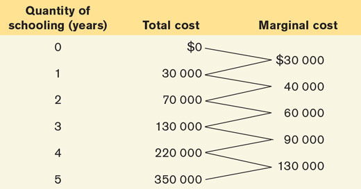
The second column also shows that the total cost of attending two years is $70 000: $30 000 for his first year plus $40 000 for his second year. During his second year in school, his explicit costs have stayed the same ($10 000) but his implicit cost of forgone salary has gone up to $30 000. That’s because he’s a more valuable worker with one year of schooling under his belt than with no schooling. Likewise, the total cost of three years of schooling is $130 000: $30 000 in explicit cost for three years of tuition plus $100 000 in implicit cost of three years of forgone salary. The total cost of attending four years is $220 000, and $350 000 for five years.
The change in Alex’s total cost of schooling when he goes to school an additional year is his marginal cost of the one-
The marginal cost of producing a good or service is the additional cost incurred by producing one more unit of that good or service.
where ΔTC is the change in total cost and ∆q is the change in quantity. For each step in Table 9-4, Δq = 1, so the marginal cost is simply the change in total cost.
Production of a good or service has increasing marginal cost when each additional unit costs more to produce than the previous one.
As already mentioned, the third column of Table 9-4 shows Alex’s marginal costs of more years of schooling, which have a clear pattern: they are increasing. They go from $30 000, to $40 000, to $60 000, to $90 000, and finally to $130 000 for the fifth year of schooling. That’s because each year of schooling would make Alex a more valuable and highly paid employee if he were to work. As a result, forgoing a job becomes more and more costly as he becomes better educated. This is an example of what economists call increasing marginal cost, which occurs when each unit of a good costs more to produce than the previous unit.
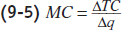
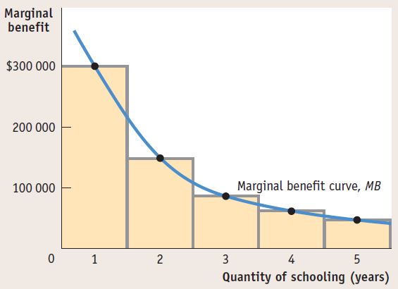
Figure 9-1 shows a marginal cost curve, a graphic representation of Alex’s marginal costs. The height of each shaded bar corresponds to the marginal cost of a given year of schooling. The red line connecting the dots at the midpoint of the top of each bar is Alex’s marginal cost curve. Alex has an upward-
The marginal cost curve shows how the cost of producing one more unit depends on the quantity that has already been produced.
Production of a good or service has constant marginal cost when each additional unit costs the same to produce as the previous one.
Although increasing marginal cost is a frequent phenomenon in real life, it’s not the only possibility. Constant marginal cost occurs when the cost of producing an additional unit is the same as the cost of producing the previous unit. Plant nurseries, for example, typically have constant marginal cost—
Production of a good or service has decreasing marginal cost when each additional unit costs less to produce than the previous one.
There can also be decreasing marginal cost, which occurs when marginal cost falls as the number of units produced increases. With decreasing marginal cost, the marginal cost line is downward sloping. Decreasing marginal cost is often due to learning effects in production: for complicated tasks, such as assembling a new model of a car, workers are often slow and mistake-
Finally, for the production of some goods and services the shape of the marginal cost curve changes as the number of units produced increases. For example, auto production is likely to have decreasing marginal costs for the first batch of cars produced as workers iron out kinks and mistakes in production. Then production has constant marginal costs for the next batch of cars as workers settle into a predictable pace. But at some point, as workers produce more and more cars, marginal cost begins to increase as they run out of factory floor space and the auto company incurs costly overtime wages. This gives rise to what we call a “swoosh”-shaped marginal cost curve—
TOTAL COST VERSUS MARGINAL COST
It can be easy to conclude that marginal cost and total cost must always move in the same direction. That is, if total cost is rising, then marginal cost must also be rising. Or if marginal cost is falling, then total cost must be falling as well. But the following example shows that this conclusion is wrong.
Let’s consider the example of auto production, which, as we mentioned earlier, is likely to involve learning effects. Suppose that for the first batch of cars of a new model, each car costs $10 000 to assemble. As workers gain experience with the new model, they become better at production. As a result, the per-
In this example, marginal cost is decreasing over batches one through four, falling from $10 000 to $5000. However, it’s important to note that total cost is still increasing over the entire production run because marginal cost is greater than zero. To see this point, assume that each batch consists of 100 cars. Then the total cost of producing the first batch is 100 × $10 000 = $1 000 000. The total cost of producing the first and second batch of cars is $1 000 000 + (100 × $8000) = $1 800 000. Likewise, the total cost of producing the first, second, and third batch is $1 800 000 + (100 × $6500) = $2 450 000, and so on. As you can see, although marginal cost is decreasing over the first few batches of cars, total cost is increasing over the same batches.
This shows us that totals and marginals can sometimes move in opposite directions. So it is wrong to assert that they always move in the same direction. What we can assert is that total cost increases whenever marginal cost is positive, regardless of whether marginal cost is increasing or decreasing.
Marginal Benefit
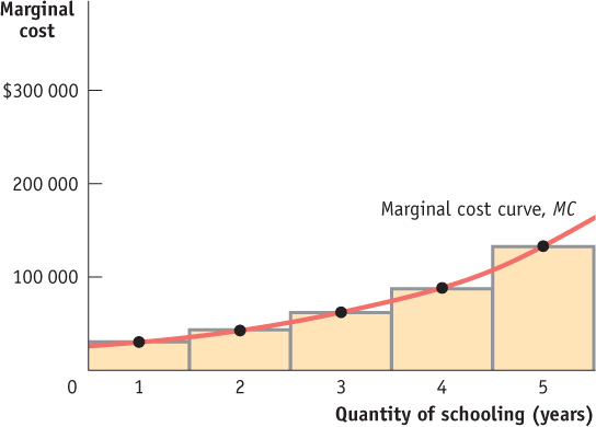
Alex benefits from higher lifetime earnings as he completes more years of school. Exactly how much he benefits is shown in Table 9-5. Column 2 shows Alex’s total benefit according to the number of years of school completed, expressed as the value of the increase in lifetime earnings. The third column shows Alex’s marginal benefit from an additional year of schooling. In general, the marginal benefit of producing a good or service is the additional benefit earned from producing one more unit.
The marginal benefit of a good or service is the additional benefit derived from producing one more unit of that good or service.
There is decreasing marginal benefit from an activity when each additional unit of the activity yields less benefit than the previous unit.
As in Table 9-4, the data in the third column of Table 9-5 show a clear pattern. However, this time the numbers are decreasing rather than increasing. The first year of schooling gives Alex a $300 000 increase in the value of his lifetime earnings. The second year also gives him a positive return, but the size of that return has fallen to $150 000; the third year’s return is also positive, but its size has fallen yet again to $90 000; and so on. In other words, the more years of school that Alex has already completed, the smaller the increase in the value of his lifetime earnings from attending one more year. Alex’s schooling decision has what economists call decreasing marginal benefit: each additional year of school yields a smaller benefit than the previous year. Or, to put it slightly differently, with decreasing marginal benefit, the benefit from producing one more unit of the good or service falls as the quantity already produced rises.
The marginal benefit curve shows how the benefit from producing one more unit depends on the quantity that has already been produced.
Just as marginal cost can be represented by a marginal cost curve, marginal benefit can be represented by a marginal benefit curve, shown in blue in Figure 9-2. Alex’s marginal benefit curve slopes downward because he faces decreasing marginal benefit from additional years of schooling.
Not all goods or activities exhibit decreasing marginal benefit. In fact, there are many goods for which the marginal benefit of production is constant—
Now we are ready to see how the concepts of marginal benefit and marginal cost are brought together to answer the question of how many years of additional schooling Alex should undertake.
Marginal Analysis
Table 9-6 shows the marginal cost and marginal benefit numbers from Tables 9-4 and 9-5. It also adds an additional column: the additional profit to Alex from staying in school one more year, equal to the difference between the marginal benefit and the marginal cost of that additional year in school. (Remember that it is Alex’s economic profit that we care about, not his accounting profit.) We can now use Table 9-6 to determine how many additional years of schooling Alex should undertake in order to maximize his total profit.
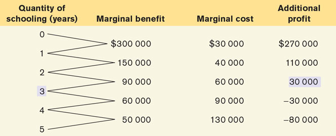
First, imagine that Alex chooses not to attend any additional years of school. We can see from column 4 that this is a mistake if Alex wants to achieve the highest total profit from his schooling—
Now, let’s consider whether Alex should attend the second year of school. The additional profit from the second year is $110 000, so Alex should attend the second year as well. What about the third year? The additional profit from that year is $30 000; so, yes, Alex should attend the third year as well. What about a fourth year? In this case, the additional profit is negative: it is –$30 000. Alex loses $30 000 of the value of his lifetime earnings if he attends the fourth year. Clearly, Alex is worse off by attending the fourth additional year rather than taking a job. And the same is true for the fifth year as well: it has a negative additional profit of –$80 000.
The optimal quantity is the quantity that generates the highest possible total profit.
What have we learned? That Alex should attend three additional years of school and stop at that point. Although the first, second, and third years of additional schooling increase the value of his lifetime earnings, the fourth and fifth years diminish it. So three years of additional schooling lead to the quantity that generates the maximum possible total profit. It is what economists call the optimal quantity—the quantity that generates the maximum possible total profit.
Figure 9-3 shows how the optimal quantity can be determined graphically. Alex’s marginal benefit and marginal cost curves are shown together. If Alex chooses fewer than three additional years (that is, 0, 1, or 2 years), he will choose a level of schooling at which his marginal benefit curve lies above his marginal cost curve. He can make himself better off by staying in school. If instead he chooses more than three additional years (4 or 5 years), he will choose a level of schooling at which his marginal benefit curve lies below his marginal cost curve. He can make himself better off by not attending the additional year of school and taking a job instead.
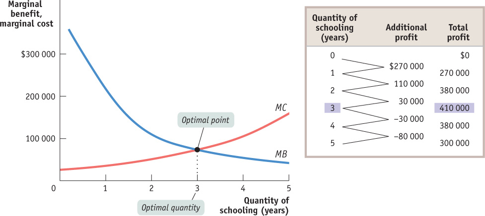
The table in Figure 9-3 confirms our result. The second column repeats information from Table 9-6, showing Alex’s marginal benefit minus marginal cost—
Alex’s decision problem illustrates how you go about finding the optimal quantity when the choice involves a small number of quantities (in this example, one through five years). With small quantities, the rule for choosing the optimal quantity is: Increase the quantity as long as the marginal benefit from one more unit is greater than the marginal cost, but stop before the marginal benefit becomes less than the marginal cost.
In contrast, when a “how much” decision involves relatively large quantities, the rule for choosing the optimal quantity simplifies to this: The optimal quantity is the quantity at which marginal benefit is equal to marginal cost.
To see why this is so, consider the example of a farmer who finds that her optimal quantity of wheat produced is 5000 bushels. Typically, she will find that in going from 4999 to 5000 bushels, her marginal benefit is only very slightly greater than her marginal cost—
According to the profit-maximizing principle of marginal analysis, when faced with a profit-
Now we are ready to state the general rule for choosing the optimal quantity—
PORTION SIZES
Health experts call it the “French Paradox.” If you think French food is fattening, you’re right: the French diet is, on average, higher in fat than the North American diet. Yet the French themselves are considerably thinner than we are: in 2011, between 9% and 11% of French adults were classified as obese, compared with 24.2% of Canadians, 30% of Mexicans, and 33.8% of Americans.
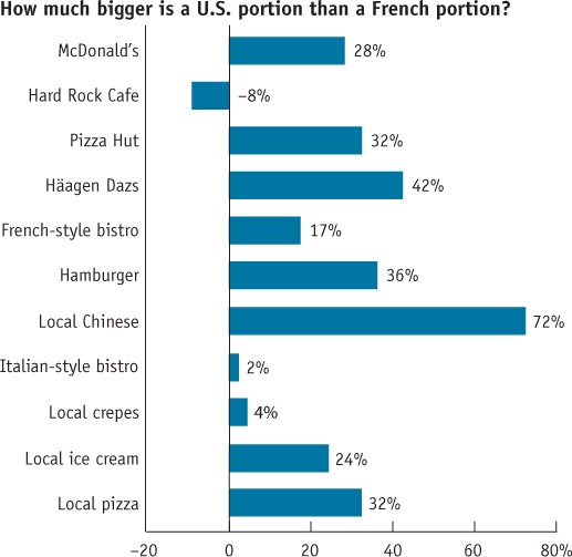
What’s the secret? It seems that the French simply eat less, largely because they eat smaller portions. This chart compares average portion sizes at food establishments in Paris, France and Philadelphia, USA. In four cases, researchers looked at portions served by the same chain; in the other cases, they looked at comparable establishments, such as local pizza parlours. In every case but one, U.S. portions were bigger, in most cases much bigger. It should be noted that while serving sizes at fast-
Why are North American portions so big? Because food is cheaper here! At the margin, it makes sense for restaurants to offer big portions, since the additional cost of enlarging a portion is relatively small. As a recent newspaper article states: “So while it may cost a restaurant a few pennies to offer 25% more French fries, it can raise its prices much more than a few cents. The result is that larger portions are a reliable way to bolster the average [price at North American] restaurants.” So if you have ever wondered why dieting seems to be a uniquely North American obsession, the principle of marginal analysis can help provide the answer: it’s to counteract the effects of our larger portion sizes.
Source: Paul Rozin, Kimberly Kabnick, Erin Pete, Claude Fischler, and Christy Shields, “The Ecology of Eating,” Psychological Science 14 (September 2003): 450–454.
Graphically, the optimal quantity is the quantity of an activity at which the marginal benefit curve intersects the marginal cost curve. For example, in Figure 9-3 the marginal benefit and marginal cost curves cross each other at three years—
A straightforward application of marginal analysis explains why so many people went back to school in 2009 through 2012: in the depressed job market, the marginal cost of another year of school fell because the opportunity cost of forgone wages had fallen.
Simple applications of marginal analysis can explain many facts, such as why restaurant portion sizes in the United States and, to some extent, Canada are typically larger than those in other countries (as was just discussed in the Global Comparison).
A Principle with Many Uses
The profit-maximizing principle of marginal analysis can be applied to just about any “how much” decision in which you want to maximize the total profit for an activity. It is equally applicable to production decisions, consumption decisions, and policy decisions. Furthermore, decisions where the benefits and costs are not expressed in dollars and cents can also be made using marginal analysis (as long as benefits and costs can be measured in some type of common units). Here are a few examples of decisions that are suitable for marginal analysis:
A producer, the retailer PalMart, must decide on the size of the new store it is constructing in Beijing. It makes this decision by comparing the marginal benefit of enlarging the store by one square metre (the value of the additional sales it makes from that additional square metre of floor space) to the marginal cost (the cost of constructing and maintaining the additional square metre). The optimal store size for PalMart is the largest size at which marginal benefit is greater than or equal to marginal cost.
Many useful drugs have side effects that depend on the dosage. So a physician must consider the marginal cost, in terms of side effects, of increasing the dosage of a drug versus the marginal benefit of improving health by increasing the dosage. The optimal dosage level is the largest level at which the marginal benefit of disease amelioration is greater than or equal to the marginal cost of side effects.
A farmer must decide how much fertilizer to apply. More fertilizer increases crop yield but also costs more. The optimal amount of fertilizer is the largest quantity at which the marginal benefit of higher crop yield is greater than or equal to the marginal cost of purchasing and applying more fertilizer.
A jewellery maker must decide on how many sets of earrings to make. Assuming they can all be sold, making more earrings increases revenue but may also drive up the marginal cost of production. The optimal level of production is the largest quantity at which the marginal benefit of production (the revenue) is greater or equal to the marginal cost of production.
MUDDLED AT THE MARGIN
The idea of setting marginal benefit equal to marginal cost sometimes confuses people. Aren’t we trying to maximize the difference between benefits and costs? Yes. And don’t we wipe out our gains by setting benefits and costs equal to each other? Yes. But that is not what we are doing. Rather, what we are doing is setting marginal, not total, benefit and cost equal to each other.
Once again, the point is to maximize the total profit from an activity. If the marginal benefit from the activity is greater than the marginal cost, doing a bit more will increase that gain. If the marginal benefit is less than the marginal cost, doing a bit less will increase the total profit. So only when the marginal benefit and marginal cost are equal is the difference between total benefit and total cost at a maximum.
A Preview: How Consumption Decisions Are Different We’ve established that marginal analysis is an extraordinarily useful tool. It is used in “how much” decisions that are applied to both consumption choices and to profit maximization. Producers use it to make optimal production decisions at the margin and individuals use it to make optimal consumption decisions at the margin. But consumption decisions differ in form from production decisions. Why the difference? Because when individuals make choices, they face a limited amount of income. As a result, when they choose more of one good to consume (say, new clothes), they must choose less of another good (say, restaurant dinners). In contrast, decisions that involve maximizing profit by producing a good or service —such as years of education or tonnes of wheat—are not affected by income limitations. For example, in Alex’s case, we assume he is not limited by income because he can always borrow to pay for another year of school. In Chapter 10 we we will see in greater detail how consumption decisions differ from production decisions—but also how they are similar.
THE COST OF A LIFE
What’s the marginal benefit to society of saving a human life? You might be tempted to answer that human life is infinitely precious. If in the real world, resources are scarce, so we must decide how much to spend on saving lives since we cannot spend infinite amounts. After all, we could surely reduce highway deaths by dropping the speed limit on highways to 60 kilometres per hour, but the cost of such a lower speed limit—in time and money—is more than most people are willing to pay.
Generally, people are reluctant to talk in a straightforward way about comparing the marginal cost of a life saved with the marginal benefit—it sounds too callous. Sometimes, however, the question becomes unavoidable.
For example, the cost of saving a life became an object of intense discussion in the United Kingdom in 1999 after a horrible train crash near London’s Paddington station killed 31 people. There were accusations that the British government was spending too little on rail safety. However, the government estimated that improving rail safety would cost more than $6 million per life saved. But if that amount was worth spending—that is, if the estimated marginal benefit of saving a life exceeded $6 million—then the implication was that the British government was spending far too little on traffic safety. In contrast, the estimated marginal cost per life saved through highway improvements was only $1.5 million, making it a much better deal than saving lives through greater rail safety.
More recently, a 2013 train derailment in Lac-Mégantic, Quebec caused explosions and fire that killed 47 people. According to reports, one possible contributing factor in this disaster was the exemption the rail company had received that allowed it to use a one-person crew rather than the usual minimum two-person crew. This exemption allowed the rail company to park an unattended train loaded with highly flammable crude oil several kilometres uphill from the town. This exemption, used to save a few hundred dollars per train shipment, resulted in 47 deaths, the destruction of most of the town’s downtown, and the release of about 7.6 million litres of crude oil. The exemption is no longer permitted on trains carrying dangerous materials in Canada.

Quick Review
A “how much” decision is made by using marginal analysis.
The marginal cost of producing a good or service is represented graphically by the marginal cost curve . An upward-sloping marginal cost curve reflects increasing marginal cost. Constant marginal cost is represented by a horizontal marginal cost curve. A downward-sloping marginal cost curve reflects decreasing marginal cost.
The marginal benefit of producing a good or service is represented by the marginal benefit curve. A downward-sloping marginal benefit curve reflects decreasing marginal benefit.
The optimal quantity, the quantity which generates the highest possible total profit, is found by applying the profit-maximizing principle of marginal analysis, according to which the optimal quantity is the largest quantity at which marginal benefit is greater than or equal to marginal cost. Graphically, it is the quantity at which the marginal cost curve intersects the marginal benefit curve.
Check Your Understanding 9-2
CHECK YOUR UNDERSTANDING 9-2
Question 9.4
For each of the “how much” decisions listed in Table 9-3, describe the nature of the marginal cost and of the marginal benefit.
The marginal cost of doing your laundry is any monetary outlays plus the opportunity cost of your time spent doing laundry today—that is, the value you would place on spending time today on your next best alternative activity, like seeing a movie. The marginal benefit is having more clean clothes today to choose from.
The marginal cost of changing your oil is the opportunity cost of time spent changing your oil now as well as the explicit cost of the oil change. The marginal benefit is the improvement in your car’s performance.
The marginal cost is the unpleasant feeling of a burning mouth that you receive from it plus any explicit cost of the jalapeno. The marginal benefit of another jalapeno on your nachos is the pleasant taste that you receive from it.
The marginal benefit of hiring another worker in your company is the value of the output that worker produces. The marginal cost is the wage you must pay that worker.
The marginal cost is the value lost due to the increased side effects from this additional dose. The marginal benefit of another dose of the drug is the value of the reduction in the patient’s disease.
The marginal cost is the opportunity cost of your time—what you would have gotten from the next best use of your time. The marginal benefit is the probable increase in your grade.
Question 9.5
Suppose that Alex’s school charges a fixed fee of $70 000 for four years of schooling. If Alex drops out before he finishes those four years, he still has to pay the $70 000. Alex’s total cost for different years of schooling is now given by the data in the accompanying table. Assume that Alex’s total benefit and marginal benefit remain as reported in Table 9-5.
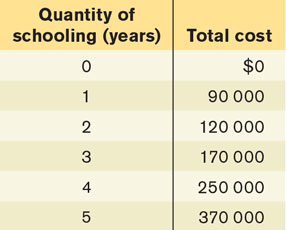
Use this information to calculate (i) Alex’s new marginal cost, (ii) his new profit, and (iii) his new optimal years of schooling. What kind of marginal cost does Alex now have—constant, increasing, or decreasing?
The accompanying table shows Alex’s new marginal cost and his new profit. It also reproduces Alex’s marginal benefit from Table 9-5.
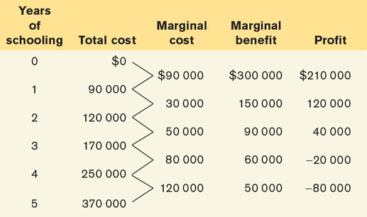
Alex’s marginal cost is decreasing until he has com-pleted two years of schooling, after which marginal cost increases because of the value of his forgone income. The optimal amount of schooling is still three years. For less than three years of schooling, marginal benefit exceeds marginal cost; for more than three years, marginal cost exceeds marginal benefit.