Chapter 7.
Overview
Generality
Thermodynamics is a tool that scientists from all fields, especially chemistry, physics, biology, earth sciences, and environmental sciences, find to be a very useful for understanding macroscopic behaviors of all variety of systems and in determining values of physical variables. The first law of thermodynamics extends the ideas introduced in the Energy-Interaction Model and casts energy conservation in ways that are particularly useful to systems involving changes in internal energies. The second law of thermodynamics, which embodies the construct of entropy, applies to all macroscopic matter, since all macroscopic matter is made up of extremely large numbers of atomic size particles. The connection of entropy to particles is taken up in the Intro Statistical Model of Thermodynamics.
Focus
Part of our focus in this model will be on developing answers to questions like the following:
Why is thermodynamics such a useful tool throughout all the sciences?
Why does almost everything you look up in a chemistry or biochemistry reference have a “∆H” associated with it? And why is it so often negative?
What the heck is “entropy,” anyway? Does the 2nd law of Thermo have anything to do with the perpetual state of my desk? My hectic life?
Why does Gibbs Energy seem to be such an important idea? And what is it that is “free” about it anyway?”
We will also get a chance to use the ideas and constructs of thermodynamics to answer some interesting questions like the following:
What is different when water evaporates from your skin on a warm summer and from the surface of a pot of nearly boiling water in an open pot on the stove?
What is the temperature of the water vapor as it leaves your skin? How much cooling does sweating produce?
How can we calculate the amount of cooling?
Model Summary
Representational Tools
Algebraic Representations
Relationship (1–3)
∆E = ∆Emechanical + ∆U
∆Ephysical system = Qin to physical system + Wdone on physical system or simply ∆E = Q + W
∆U = ∆Ebond + ∆Ethermal + ∆Eatomic + ∆Enuclear
∆U = Q + W
in differential form: dU = dQ + dW
and for simple fluids: dU = dQ – PdV
and for fluid processes along reversible paths: dU = TdS – PdV
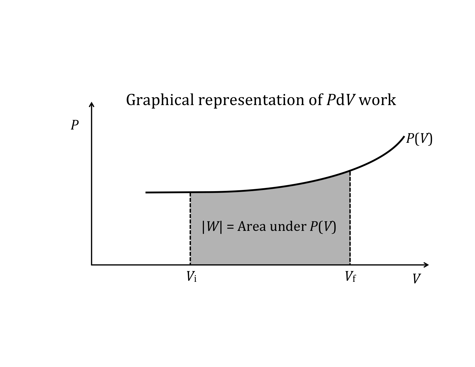
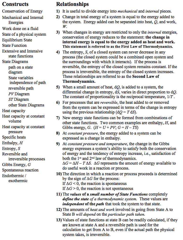
Expression for work done on a fluid
or in differential form: dW = -P(V) dV
Relations 4–6
The Second Law of Thermodynamics
In a closed system, ∆S ≥ 0
Extension of the concept of heat capacity
Heat Capacity
Heat Capacity at Constant Volume and Constant Pressure (with ∆EBond = 0)
Relations 7–10
Enthalpy
H = U + PV, At constant pressure, ∆H = Q
Gibbs Energy
G = H - TS, At constant pressure and temperature, ∆G = ∆H – T ∆S
If ∆G < 0, the process is spontaneous
If ∆G > 0, the process is not spontaneous
If ∆G = 0, the forward and reverse directions are in equilibrium
State Functions: Ideal Gas Law: PV = nRT or PV = N kBT
Graphical Representations
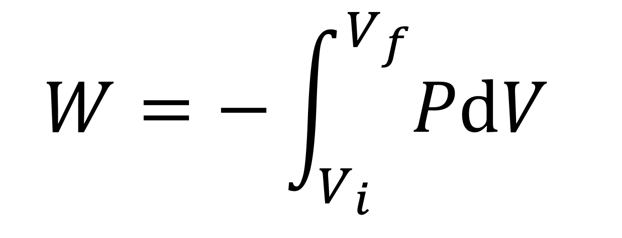
Two identical states, A & B shown on both State Diagrams, but the processes that take the physical system from A to B are different in the two State Diagrams.
Elaboration
Expanded Definitions of New Model Constructs
Work done on a fluid
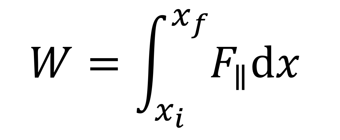
In the Energy-Interaction Model we defined work, W as the product of the unbalanced force acting on an object parallel to the displacement of the object, ∆x.
The more general expression that takes into account the fact that F|| can change as the object moves (i.e., F|| can be a function of x is
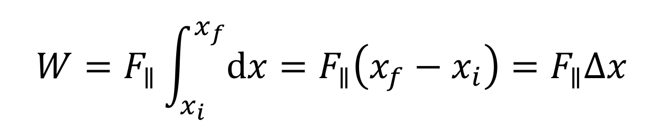
There are several special cases that are worth noting. First, the force can be constant. Thus, F||(x) = F||, and F||(x) can be taken outside the integral to yield our previous result:
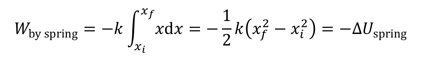
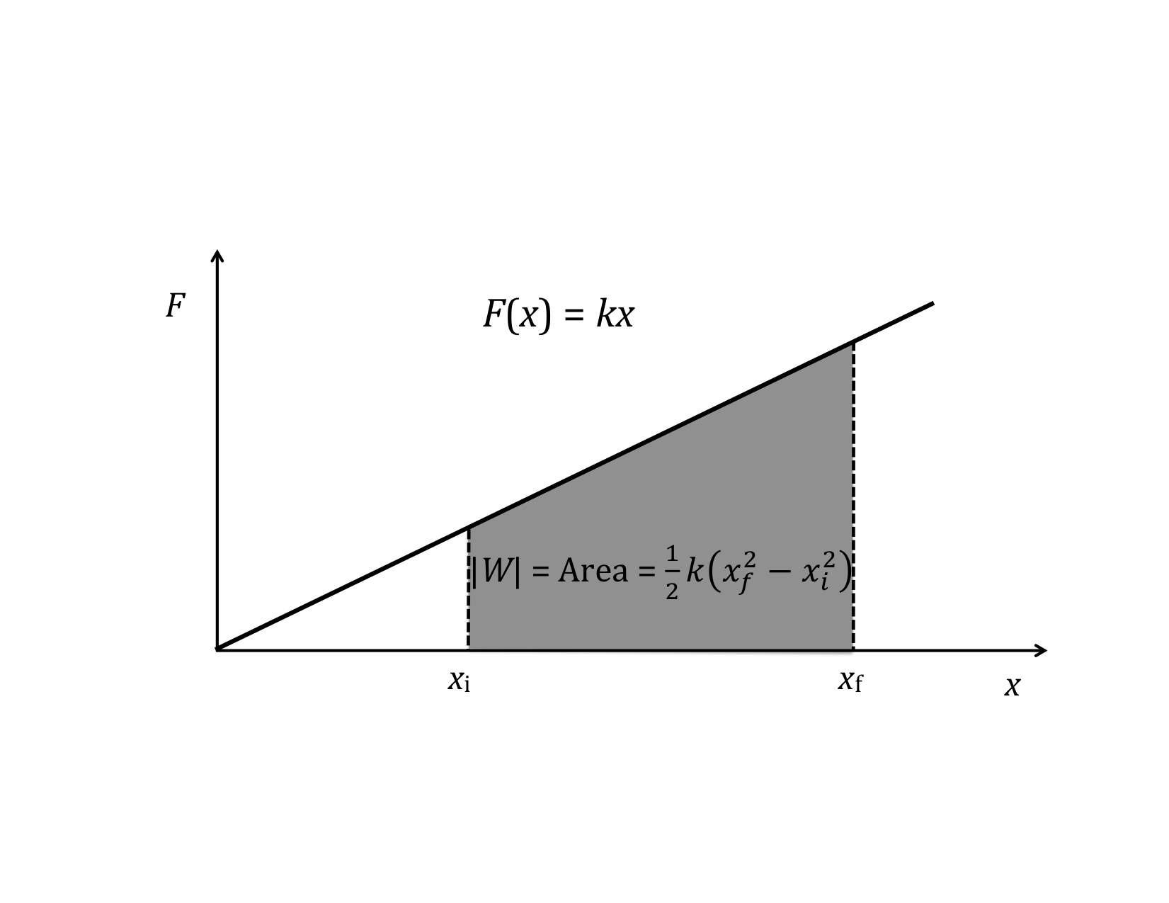
The next simplest case is when the force is a linear function of x. For instance, the force by a spring is F||(x) = -kx, as for a spring. Work then becomes
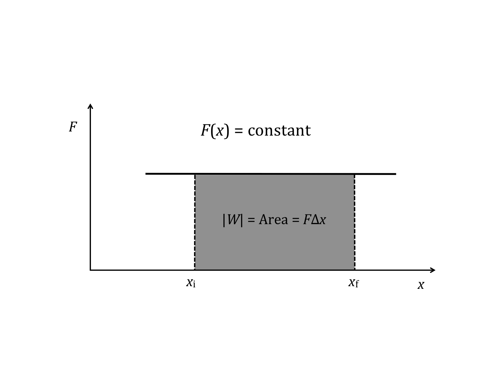
If F||(x) is plotted as a function of x, there is a very simple interpretation of the definite integral in the above equation: the work, W, is simply the area under the F||(x) curve.

Graphical interpretation of the two special cases:
and
Rather than the integral expression for work, it is often convenient to use a differential expression. That is, we want to talk about the small increment of work corresponding to the product of the parallel component of force and the differential increment of distance, dx.
dW = F||(x) dx
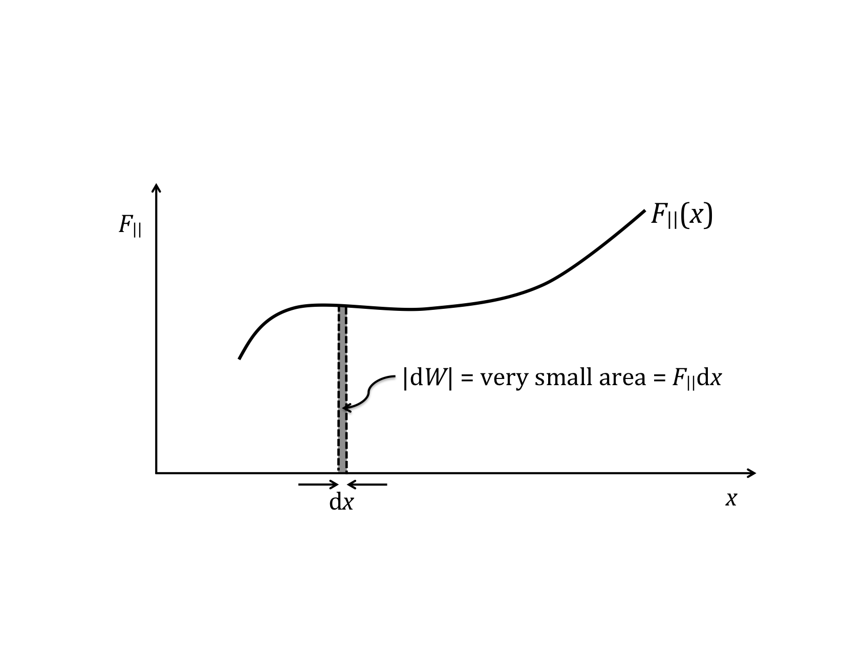
This expression for the incremental work fits nicely with the graphical representation of work and the graphical interpretation of the definite integral. If you do not remember this from your calculus class, you might want to go back and review it over the next couple of weeks. (The graphical interpretations of derivatives and integrals are two of the those important concepts that you should take away from calculus, i.e., things you remember for the rest of your life.)
Now we are ready to consider the work done on a fluid.
We now have general expressions for work in terms of forces and distances moved. But when you push on a fluid (i.e., a liquid or a gas), the magnitude of the force depends on how hard you push as well as the area of your hand. It depends on a property of the fluid–a property we call pressure.
Pressure turns out to be an important and useful property of a fluid. It has to do with how much the fluid is “squeezed”. The force exerted on a fluid by an object of cross-sectional area A is proportional to the pressure P and area A and is directed in a direction perpendicular to A.
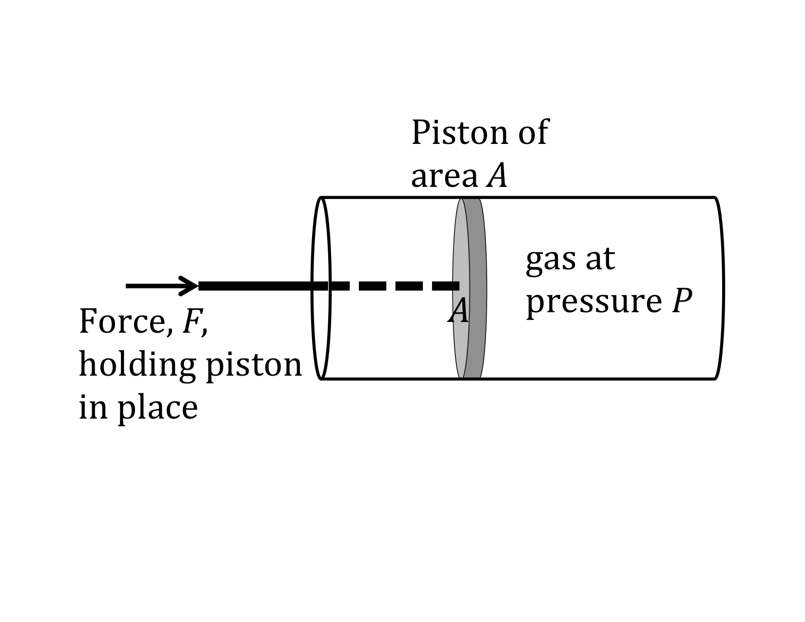
The force pushing the movable piston to the right is equal (when there are no accelerations) to the force the fluid contained in the cylinder exerts on the piston to the left. The magnitude of this force is not a definition of pressure, but simply the relation of force to pressure
The units of pressure are force per area, which is also energy per volume.
Useful reference information
In SI,
Our previous expressions for work were in terms of the linear distance. When dealing with fluids, it is useful to make a change of variables from x to V. The relation between the differentials dV and dx is illustrated in the figure.
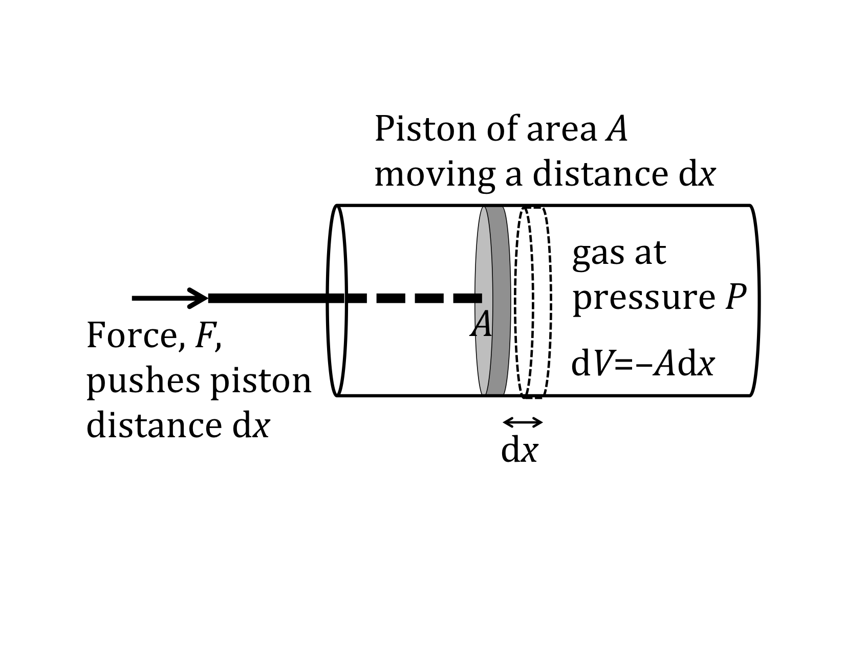
Note: The reason for the minus sign in front of dV is because the volume gets smaller as “x” increases in the positive direction to the right.
substituting -dV/A for dx and
the integral becomes
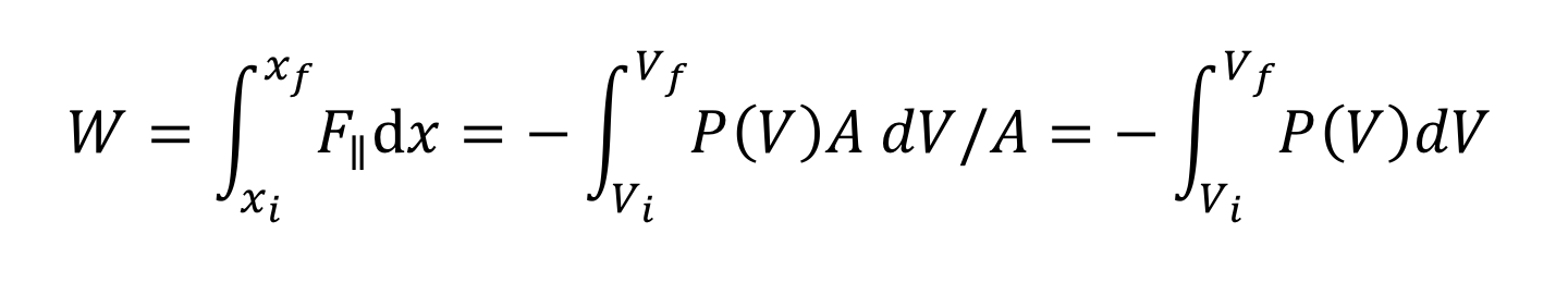
or
This is the expression for the work done on a fluid when it is compressed from a volume Vi to a volume Vf. Note that the minus sign in front of the integral ensures that work comes out positive (since PdV is negative). If instead of being compressed, the volume expands, the work done on the fluid will be negative. Equivalently, we can say that the fluid does positive work on some other physical system.
In differential form, the work done when changing the volume of a fluid is
To proceed further, we need to know how the pressure, P, depends on the volume, V. For gases that are not too dense, we can use the ideal gas law, which relates the volume, pressure, temperature T, and number of gas particles N (or number of moles n):
where kB is Boltzmann’s constant and R is the gas constant familiar from chemistry.
R = 8.314 J / mol•K
The ideal gas law states that pressure and volume are not uniquely related, but depend on the temperature. Therefore, the work done when compressing a gas will depend on how temperature changes as the pressure and volume change. That is, it takes different amounts of work to compress a gas, depending on how the temperature varies during the compression, as heat is or is not allowed to enter the system. PV diagrams and a new way of stating conservation of energy will allow us to determine the contributions of work and heat to changes in systems.
State of a Physical System, Equilibrium State
One aspect of thermodynamics that we will pursue is how systems evolve from one state to another. To understand this we need to be able to describe the initial and final endpoint states and to describe the process for getting from one to the other. In describing individual states, we can use certain variables that have unique values for any state. These variables are called “state variables.” For example, an ideal gas in a particular state will have one value for P, V, T, and U. Relationships between these variables are expressed in “equations of state.” You are already familiar (from chemistry) with one equation of state – the ideal gas equation (PV = nRT). As a system changes, due to heat or work being added or removed, the values of these state variables will change.
Previously we found it was useful to use energy-system diagrams to help us focus on changes of energy. These energy-system diagrams were a useful representational tool. To describe changes in state variables as a system undergoes change, we can use a different representational tool: state diagrams. A state diagram is a graph of one state variable plotted as a function of another state variable for a particular process. Because it is frequently the case that two state variables completely determine the “state” of the system, a two dimensional state diagram can be a very useful representational tool. Often, the pressure, P, and volume, V, are chosen to be the two state variables. Another useful pair is entropy and temperature.
State Diagrams
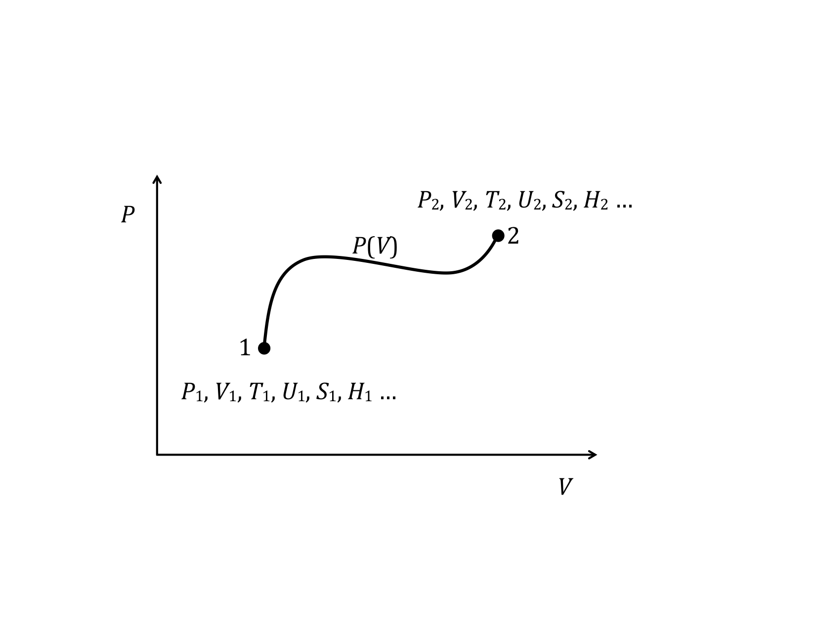
One reason the two-variable state diagram is such a useful representation, is because it is possible to easily follow the path a system takes as it undergoes the process for going from the initial to the final state. By path, we mean the continuous line of intermediate states that a system passes through, as it moves from an initial to a final state. The PV diagram below shows one of the infinite number of possible paths connecting state-1 with state-2.
Equilibrium State
It makes no sense to try to represent a state of a system on state diagram, unless the system is in equilibrium. The state variables, which are macroscopic variables, must have unique values that are the same throughout the system. Likewise, it makes no sense to talk about a particular path along a state diagram unless all the intermediate states are equilibrium states as well. This is not to say that a real physical system can’t go from one state, say state-1 in the example above to state 2 and not follow a set of intermediate states that are equilibrium states. In fact, most processes do not follow a path that continuously moves along a set of equilibrium states. It is just that we can’t show the path if it does not pass through a series of equilibrium states. The end points, however, are well defined, regardless of how the system gets from the initial to the final equilibrium state. The system can start in an equilibrium state and end up in an equilibrium state and never be in an equilibrium state along the way.
PV Diagram
We will find many uses for PV-diagrams in connection with understanding the energy exchanges that take place as thermodynamic systems undergo change. One of the most important things we have already seen is that the area under a PV-curve represents the work done on or by the system during a volume change. This work, in turn, is directly related to heat transfer and changes in the internal energy of the system.
Heat Capacity at Constant V and at Constant P
Any heat capacity measurement consists of adding a known amount of heat to a substance and measuring the temperature change.
For now, we consider only substances whose only internal energies are bond and thermal and we specifically make the heat capacity measurement at temperatures where bond energy changes do NOT occur. But there is still an issue as to whether the system we are interested does work (or has work done on it) during the process of adding heat to make the heat capacity measurement. Consequently, it is common to define to specific processes: one at constant volume, so that no work is done, and the other at constant pressure, so, especially with gases, there is definitely work involved. We will come back to this shortly at the end of the discussion on relationships between the constructs.
A New State Function: Enthalpy, H
A state function depends only on the condition of a system at a particular time. It does not depend on how it got to be in that condition. The state function we have been dealing with all quarter is, of course, energy. The energy of a system depends only on the values of some state variables at the particular time. Work and heat are not state variables. They are processes. Their values depend on how a system is changed. This distinction is critically important to understand.
If you look up values of most thermal properties such as heats of fusion, vaporization, or combustion, you will often find them tabulated as changes of enthalpy, expressed by the symbol ∆H. Enthalpy, like energy, is a state function. It depends only on the values of certain parameters at that time, but does not depend on how the system got to those values. We will see how this comes about in the relationship section shortly.
Another New State Function: Entropy, S
We will also take a close look at another state function, the entropy, S. Entropy is directly connected to the statistical behavior of large numbers of particles. In addition to using the statistical approach, we will examine entropy from the perspective of thermodynamics, to see how it is related to other thermodynamic variables. Using both approaches will help us to make better sense out of what is often a very confusing and mysterious concept.
Reversible Process or Reversible Path
One way to think about reversibility is simply to ask, can a system move along a path and then stop and have the process that took it along the path “run backwards” and get back to exactly the same state by following along the exact same path? For this to happen two conditions have to be met. First, there can be no friction. Friction causes energy to be transferred to thermal energy systems, which can never be completely “gotten back out” of thermal systems into mechanical systems. Second, there can be no heat transfers across finite temperature differences. This last statement is a little hard to handle. The only way to have heat transfers is to have temperature differences. One way to think about this is to say to yourself, “Well, I will create just a little bitty temperature difference and wait a long time for the heat to transfer, but there will never be very much of a temperature difference.” If you have enough patience, you can make it almost reversible. So in real life, there are no truly reversible processes, but it is possible to come fairly close. And, you can certainly calculate along reversible paths, which is the real reason for this distinction.
Discussion of the Model Relationships
- It is often useful to divide all energy into mechanical and internal pieces
- Change in total energy of a system is equal to the energy added to the system. Energy added can be separated into heat, Q, and work, W.
- When changes in energy are restricted to only the internal energies, conservation of energy reduces to the statement: the change in internal energy is equal to the energy added as heat and work. This statement is referred to as the First Law of Thermodynamics.
Allowing for a transfer of energy into a physical system from outside the system as either heat or work or both, we can express conservation of energy as:
which actually means ∆Ephysical system = Qin to + Wdone on
This equation is always true as long as we interpret ∆E to include all changes of energy associated with the physical system and we mean by Q and W the addition of energy as heat or as work to the system when Q and W are positive. (A negative Q or W means that energy is removed from the system.)
where ∆U = ∆Ebond + ∆Ethermal + ∆Eatomic + ∆Enuclear and is called the change in internal energy. Eatomic includes changes in the atomic states of atoms that are not involved in chemical bonds. In normal chemical reactions and physical phase changes, there are no changes in nuclear energies, so the last term is zero.
If there are no changes in Emechanical, then the expression representing conservation of energy for a particular physical system becomes the familiar relation used by physicists and chemists known as the first law of thermodynamics:
In chemistry, the 1st law of thermodynamics at constant pressure is typically written as
The subscript “rxn” signifies that this is a change in energy due to a reaction and the lower case “q” signifies that heat is not a state function, but rather a transfer of energy. The work is expressed explicitly as -P∆V, since only this kind of work is assumed to occur. Rest assured, however, that we are talking about exactly the same thing. You should practice “seeing through or seeing past” the particular symbols to the content represented by an equation. These last two equations for ∆U are perfect examples of this point. Do you look at them and see two different strings of symbols to memorize, or do you immediately recognize them as expressing the same physical content?
It is sometimes useful to write the first law of thermodynamics in differential form:
(dQ is interpreted here to be a small transfer of energy, rather than a true differential)
- The entropy, S, of a closed system can never decrease in any process (the closed system could be a combined open system and the surroundings with which it interacts). If the process is reversible, the entropy of the closed system remains constant. If the process is irreversible, the entropy of the closed system increases. These relationships are referred to as the Second Law of Thermodynamics.
- When a small amount of heat, dQ, is added to a system the differential change in entropy, dS, varies in direct proportion to dQ. The constant of proportionality is the reciprocal temperature, 1/T . (dS = dQ/T).
- For processes in which all work is reversible, the heat added to or removed from the system can be expressed in terms of the change in entropy using the previous relationship (dQ = T dS).
The restriction of the reversible process applies only to calculating ∆S (using ∆S = Q/T or dS = dQ/T) as a system moves from one state to another. The actual change in ∆S of the system is the same, regardless of whether the change is reversible or not. That is the meaning of S being a state function. But to calculate ∆S, we must move along a hypothetical path reversibly. This is the beauty or “magic” of thermodynamics: we can calculate values of changes in state functions for very complicated processes by imagining that we move the system between the two states in a manner that makes it easy to do the calculations. But the answers we get for the changes in the state functions using this approach are the same even when the system doesn’t actually change in this way!
Closer Look at Entropy from a thermodynamic viewpoint
The fundamental relationship between entropy and energy is the following. Imagine adding heat to a system reversibly, i.e., no friction occurs and no energy is transferred as heat across a finite temperature difference. Under these conditions there is a change in entropy (entropy is created or destroyed) according to the following relationship:
Now S is a state variable, so ∆S = Sf - Si
For constant T, T ∆S = Q
or ∆S = Q/T (reversible process, constant T)
If Q is positive (meaning that heat is added to the system) ∆S is positive. On the other hand, if heat is removed, the entropy is reduced. We also see from the above relationship that the SI units of entropy are joules per kelvin.
Since ∆S is a state variable and depends only on the initial and final state, we should be able to directly express it as a function of other state variables. We can use the first law of thermodynamics to do this.
Substituting this into the our expression for entropy, dS = dQ / T, we get:
If the temperature is constant, then we can also write
Experimentally, the most direct route to the determination of values of ∆S is through heat capacity data. In general, C = dQ/dT, so
and
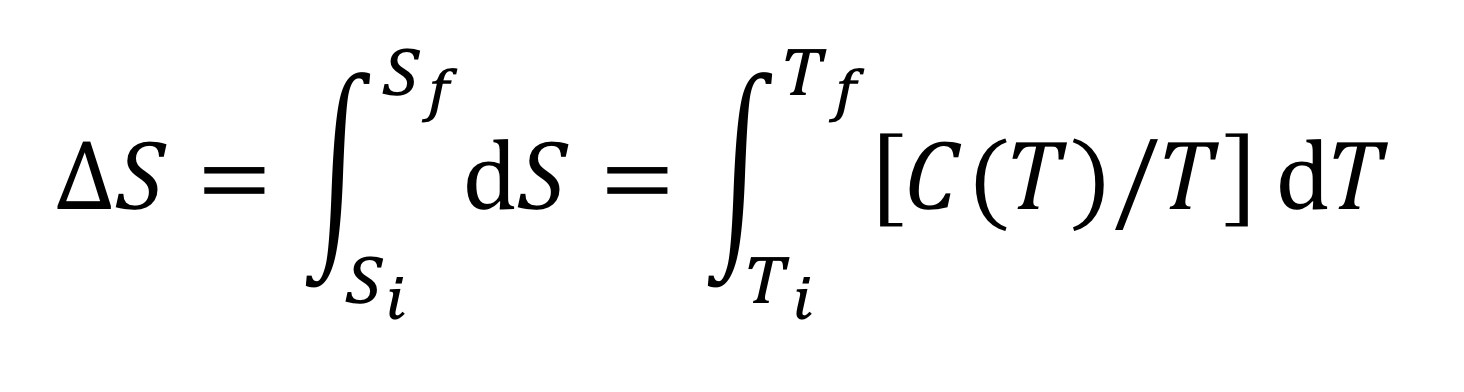
Either Cp or Cv can be used in the above relation. If Cv is used, the two state variables describing the system are T and V (V constant) and if Cp is used, the two state variables describing the system are T and P (P constant).
If C(T) is approximately constant over the temperature range in question, it can be pulled out of the integral and we have the useful result
- New energy state functions can be formed from combinations of other state functions. Two common examples are enthalpy, H, and Gibbs energy, G.
(H = U + PV; G = H – TS) - At constant pressure, the energy added to a system can be expressed as a change in enthalpy (Q = ∆H).
This is a very useful relationship! This is because so much experimental work is done in open containers at one atmosphere of pressure. This is worth looking at more closely to see how it comes about.
H = U + PV
Note that the three variables that define H are all themselves state variables.
We note for future reference that P is an energy density, which, when multiplied by volume, is an energy. Why would a function equal to the internal energy plus the product of the two state variables pressure and volume be useful? As with energy, it is the changes in H that occur during a process that are important. Changes in enthalpy are most useful under certain conditions: specifically, situations in which pressure is held constant. Chemists and biologists conduct many of their experiments (any reaction carried out in a container open to the atmosphere) under constant pressure.
The following derivation shows why enthalpy is a convenient variable when considering changes occurring under constant pressure:
For ∆U we can substitute the expression for internal energy we obtained from the first law of thermodynamics (at constant pressure): ∆U = Q - P∆V. This gives us
So at constant pressure, the enthalpy change during a reaction is simply equal to the heat entering the system. Likewise, if a phase change is allowed to occur at constant pressure, the heats of melting and vaporization are simply equal to the changes in enthalpy. So now we see why heats of fusion and vaporization are often listed as changes in enthalpies. When you measure the energies transferred as heat during a phase change at constant pressure, you are directly measuring the change in the state function H. A negative ∆H means heat is transferred out, and the reaction is exothermic. A positive ∆H means heat is transferred in and the reaction is endothermic.
∆H > 0 endothermic
It is because dH = dQ (constant pressure and only PV work) for the conditions so common in chemistry and biochemistry, and technology in general, that enthalpy is so useful. Most measurements are carried out at constant pressure, and for many systems, the only work involved comes from compressing or expanding a gas.
- At constant pressure and temperature, the change in the Gibbs energy expresses a system’s ability to satisfy both the conservation of energy and the tendency of entropy increase, i.e., satisfaction of both the 1st and 2nd law of thermodynamics.
∆G = ∆H – T ∆S. ∆G represents the amount of energy available to do useful work in a reaction or process that is carried out at constant P and T. Historically, this was called “free energy.” - The direction in which a reaction or process proceeds is determined by the sign of ∆G for the process:
If ∆G < 0, the reaction is spontaneous
If ∆G > 0, the reaction is not spontaneous
Note: A full discussion of Gibbs Energy is included in the discussion of the Intro Statistical Model of Thermodynamics: - The values of a small number of State Functions completely define the state of a thermodynamic system. These values are independent of the path that took the system to that state.
- The amounts of heat and work involved in going from State A to State B will depend on the particular path taken.
- Values of state functions at state B can be readily calculated, if they are known at state A, because a reversible path can be used for the calculation to get from A to B, even if the actual path the physical system takes, is irreversible.
Comments on 12. and 13.
The end points define the initial and final states. Those states do not depend on the path taken. All real processes have some irreversibility associated with them. However, it is usually possible to move along a path on an appropriate state diagram that is reversible, and thus possible to calculate the changes in the various state variables. So, calculations along reversible paths can allow you to find the values of the state variables. But the point of relationship (12) is that the split between the amount of energy transferred as heat and transferred as work will depend on the actual path taken, as well as the amount of irreversibility in the real process.
More on Heat Capacities
Under the assumption that there are no bond energy changes and the only energy systems are the thermal and bond systems, the first law of thermodynamics reduces to
dEth = dQ + dW, since Ebond = 0
Solving for dQ and differentiating with respect to T we obtain a general expression for the heat capacity in terms of our model:
Previously, we wanted the constant volume heat capacity. In that case, the dW/dT term was zero, so we had for constant volume:
For constant pressure, the work term is not zero, so we need to evaluate it for the particular substance we are concerned about.
The first step is to write dW as -PdV, since we are concerned with fluids (liquids and gases). The expression for Cp then becomes
Cp = Cv + PdV/dT
To go any further we need to evaluate dV/dT, which will depend on the substance. We will evaluate this when we get to the Ideal Gas Model.