Section 1: Aggregate Expenditures

Gross domestic product (GDP) is measured by spending or income. Using the spending approach, GDP is equal to aggregate expenditures (AE). Therefore:

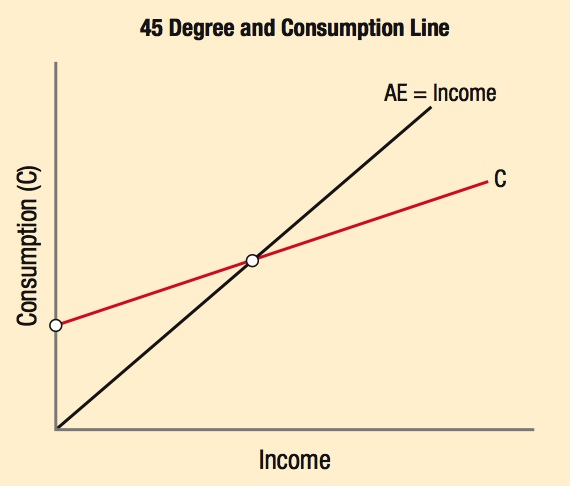
The 45° line shows where total spending (AE) equals income. No borrowing or saving exists.

The consumption line (C) starts above the origin on the vertical axis (even with no income, one still consumes by borrowing). As income increases, consumption rises, but not as fast as income (the slope of C depends on the MPC).

When C crosses AE, spending equals income (on the 45° line). When C is below the AE line, saving is positive.

Investment spending fluctuates much more than consumption year to year.

Disposable income, Y_D, is income after all taxes have been paid. Disposable income can either be spent (C) or saved (S). Thus, Y_D = C + S.

The portion that is consumed or saved is an important concept in the aggregate expenditures model:

Marginal propensity to consume (MPC) = ΔC/ΔY_D

Marginal propensity to save (MPS) = ΔS/ΔY_D

MPC + MPS = 1 (all money is either spent or saved)

Even with little to no income, college students still consume goods and services, often by borrowing against future income.

Determinants of Consumption and Saving

The aggregate expenditures model states that income is the main determinant of consumption and saving. But other factors also can shift the consumption schedule, such as:

• Wealth
• Expectations
• Household debt
• Taxes

Determinants of Investment Demand

Investment demand is assumed to be independent of income, but certain factors can shift investment demand, such as:

• Expectations
• Technological change
• Operating costs
• Capital goods on hand

Section 2: Simple Aggregate Expenditures Model

Ignoring government spending and net exports, aggregate expenditures (AE) are the sum of consumer and business investment: AE = C + I. Because AE also equals C + S at equilibrium, this means that savings = investment.

The multiplier effect occurs when a dollar of spending generates many more dollars of spending in the economy.

The multiplier is equal to:

1/(1 − MPC) or 1/MPS.

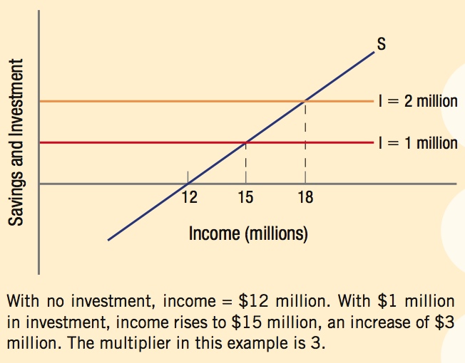
With no investment, income = $12 million. With $1 million in investment, income rises to $15 million, an increase of $3 million. The multiplier in this example is 3.

Section 3: The Full Aggregate Expenditures Model

Government spending affects the economy just like any other spending, and so does spending by foreign consumers (exports). In the full aggregate expenditures model, all forms of spending are analyzed, including C, I, G, and (X−M).

If the multiplier for an economy is 5, a $1 million increase in investment increases income by $5 million. The same effect occurs with a $1 million increase in government spending or $1 million increase in net exports. Essentially, spending is spending, no matter where it comes from.

A general way to analyze policies that increase or decrease aggregate output is to categorize activities as either an injection or a withdrawal:

Injections increase spending in an economy, and include investment (I), government spending (G), and exports (X).

Withdrawals decrease spending in an economy, and include savings (S), taxes (T), and imports (M).

In equilibrium, all injections must equal all withdrawals:

Whenever the economy moves away from its full employment equilibrium, one of two gaps is created:

Recessionary gap: The increase in aggregate spending (that is then multiplied) to bring a depressed economy to full employment.

Inflationary gap: The reduction in aggregate spending (again expanded by the multiplier) needed to reduce income to full employment levels.

Purchasing an American-made car injects spending into the economy, and the economic benefits are enhanced by the multiplier.

Purchasing a foreign-made car, however, results in a withdrawal because money leaves the country, and this effect is compounded by the multiplier.