Fiscal Policy and Aggregate Demand
When an economy faces underutilization of resources because it is stuck in equilibrium well below full employment, we saw that increases in aggregate demand can move the economy toward full employment without generating excessive inflation pressures. The recent recession provided evidence of this effect. However, in normal times, influencing aggregate demand brings with it a tradeoff: Output is increased at the expense of raising the price level.
In contrast, consider decreasing aggregate demand. When the economy is in an inflationary equilibrium above full employment, contracting aggregate demand dampens inflation but leads to another tradeoff: unemployment. Before we examine the theory behind how government actually goes about influencing aggregate demand by using fiscal policy, let’s take a brief look at what categories of spending fiscal policy typically alters.
Discretionary and Mandatory Spending
discretionary spending The part of the budget that works its way through the appropriations process of Congress each year and includes such programs as national defense, transportation, science, environment, and income security.
The federal budget can be split into two distinct types of spending: discretionary and mandatory. Discretionary spending is the part of the budget that works its way through the appropriations process of Congress each year. Discretionary spending includes such programs as national defense (primarily the military), transportation, science, environment, income security (some welfare programs and a large portion of Medicaid), education, and veterans benefits and services. As Figure 1 shows, discretionary spending is now under 40% and has steadily declined as a percent of the budget since the 1960s, when it was over 60% of the budget.
FIGURE 1
Discretionary and Mandatory Federal Spending Mandatory spending includes programs authorized by law (also called entitlements) such as Social Security, Medicare, and the Supplemental Nutrition Assistance Program. Mandatory programs do not go through the normal Congressional appropriations process and have been growing. Discretionary programs are authorized each year by the appropriations process of Congress and include national defense, transportation, environment, and education spending. Discretionary spending has been steadily declining as a percent of the budget.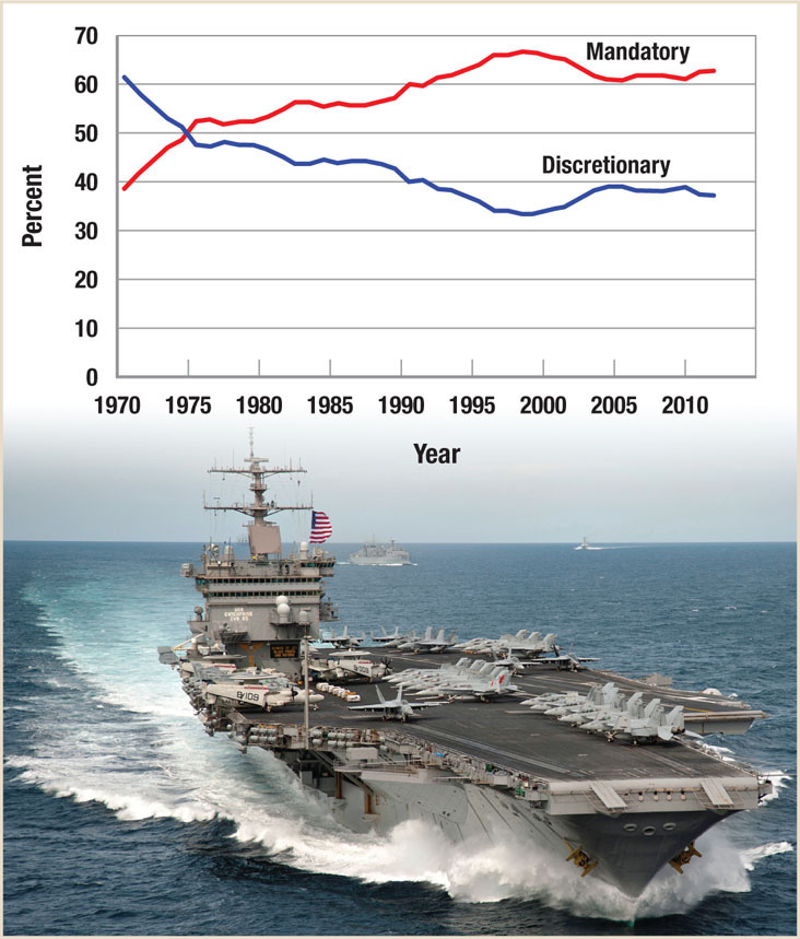
mandatory spending Spending authorized by permanent laws that does not go through the same appropriations process as discretionary spending. Mandatory spending includes such programs as Social Security, Medicare, and interest on the national debt.
Mandatory spending is authorized by permanent laws and does not go through the same appropriations process as discretionary spending. To change one of the entitlements of mandatory spending, Congress must change the law. Mandatory spending includes such programs as Social Security, Medicare, part of Medicaid, interest on the national debt, and some means-tested income-security programs, including SNAP (Supplementary Nutrition Assistance Program; formerly known as the Food Stamp Program) and TANF (Temporary Assistance to Needy Families). This part of the budget has been growing, as Figure 1 illustrates, and now accounts for over 60% of the budget.
Even though discretionary spending is only 37% of the budget, this is still roughly $1.3 trillion, and the capacity to alter this spending is a powerful force in the economy. Therefore, we are mainly concerned with discretionary spending when we consider fiscal policy.
Discretionary Fiscal Policy
discretionary fiscal policy Involves adjusting government spending and tax policies with the express short-run goal of moving the economy toward full employment, expanding economic growth, or controlling inflation.
The exercise of discretionary fiscal policy is done with the express goal of influencing aggregate demand. It involves adjusting government spending and tax policies to move the economy toward full employment, encouraging economic growth, or controlling inflation.
Some examples of the use of discretionary fiscal policy include tax cuts enacted during the Kennedy, Reagan, and George W. Bush administrations. These tax cuts were designed to expand the economy under the belief that people would spend their tax savings, both in the near term and the long run—they were meant to influence both aggregate demand and aggregate supply. Tax increases were enacted under the George H. Bush and Clinton administrations in the interest of reducing the government deficit and interest rates. The Roosevelt administration used increased government spending, although small amounts by today’s standards, to mitigate the impact of the Great Depression.
Government Spending Although discretionary fiscal policy can get complex, the impact of changes in government spending is relatively simple. As we know, a change in government spending or other components of GDP will cause income and output to rise or fall by the spending change times the multiplier.
This is illustrated in Figure 2 with the economy initially in equilibrium at point e, with real output equaling Q0. If government spending increases, shifting aggregate demand from AD0 to AD1, aggregate output will increase from Q0 to Qf. Because the short run aggregate supply curve is upward sloping, some of the increase in output is absorbed by rising prices, reducing the pure spending multiplier discussed in earlier chapters.
FIGURE 2
The Multiplier and Government Spending The economy is initially in equilibrium at point e. As new government spending works its way through the economy round-by-round, both income and output are multiplied, but price increases absorb some of the increase in AD. Once the economy reaches full employment (point a), price increases absorb all of the increase in AD.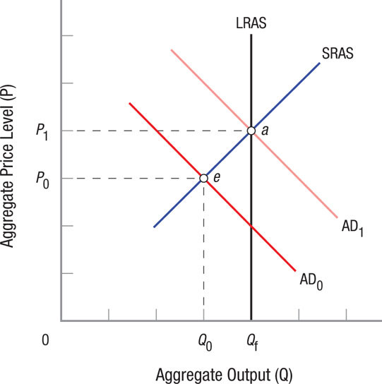
Once the economy reaches full employment (point a), further spending is not multiplied as the economy moves along the LRAS curve, and price increases absorb it all. Finally, keep in mind that the multiplier works in both directions.
Taxes Changes in government spending modify income by an amount equal to the change in spending times the multiplier. How, then, do changes in taxes affect the economy? The answer is not quite as simple. Let’s begin with a reminder of what constitutes spending equilibrium.
When the economy is in equilibrium,
GDP = C + I + G + (X − M)
At equilibrium, all spending injections into the economy equal all withdrawals of spending. To see why, let’s simplify the above equation and begin with only a private economy, eliminating government (G) and the foreign sector, or net exports (X − M). Thus,
GDP = C + I
Gross domestic product (GDP) is equal to consumer plus business investment spending. Without government and taxes, GDP is just income (Y), therefore
Y = C + I
or, subtracting C from each side of the equation,
Y − C = I
Now, income minus consumption (Y − C) is just saving (S), therefore at equilibrium,
S = I
This simple equation represents a very important point: At equilibrium, injections (in this case, I) are just equal to withdrawals (S in this instance). Investment represents spending where saving is the removal of income from the spending and income stream.
Now, without going through all of the algebra, when we add government spending (G), taxes (T), and the foreign sector (X − M) to the equation, we have just added some injections (G) and (X) and subtracted some withdrawals (T) and (M), thus the equilibrium equation becomes
I + G + X = S + T + M
With this equation in hand, let’s focus on taxes. When taxes are increased, money is withdrawn from the economy’s spending stream. When taxes are reduced, consumers and businesses have more to spend. Disposable income is equal to income minus taxes (Y − T).
Because taxes represent a withdrawal of spending from the economy, we would expect equilibrium income to fall when a tax is imposed. Consumers pay a tax increase, in part, by reducing their saving. If we initially increase taxes by $100, let’s assume that consumers draw on their savings for $25 of the increase in taxes. Because this $25 in savings was already withdrawn from the economy, only the $75 in reduced spending gets multiplied, reducing the change in income. The reduction in saving of $25 dampens the effect of the tax on equilibrium income because those funds were previously withdrawn from the spending stream. Changing the withdrawal category from saving to taxes does not affect income. A tax decrease has a similar but opposite impact because only the MPC part is spent and multiplied, and the rest is saved and thus withdrawn from the spending stream.
How Big Was the Stimulus Multiplier, Really?
President Obama’s $787 billion 2009 stimulus package set off a flurry of discussion among economists about the actual size of spending and tax multipliers. It is one thing in our simple models to show that these multipliers exist and assert the value based on the MPC (a multiplier of 4 in our model with an MPC of 0.75). But the economy is a complex machine and there are various leakages that keep the multiplier from reaching its theoretical Keynesian “depression” potential. Leakages are funds that do not find their way into the domestic consumption-income multiplication stream.
One important leakage is taxes. Income generated from one person’s consumption is taxed, reducing the amount available for further consumption and income generation. Another important leakage is purchases of imports; when consumers buy imported goods, that money flows overseas and is not multiplied here. Both taxes and imports withdraw money from the spending stream, reducing the actual value of the multiplier. This explains why Congress and the president included a number of “Buy American” provisions in the 2009 stimulus plan.
What empirical value best represents the short-term stimulus multiplier? That is not an easy question to answer because many factors influence an economy’s output, such as the trend in the business cycle. Therefore, it is difficult to narrow the effects of a specific government injection, such as the 2009 stimulus, from other factors that play a role.

Still, a number of empirical studies have attempted to estimate the multiplier and its effect on the economy. Conclusions from these studies ranged from the stimulus having a substantial effect on the economy’s recovery to having virtually no effect at all. Looking more closely at the results, however, revealed more areas of consensus. For example, most studies showed the stimulus having a positive effect on employment, and that multipliers varied depending on the type of spending used. Spending on infrastructure and low-income assistance, for example, generally showed a higher multiplier than money given to states for education and law enforcement. The latter is likely because states may have substituted stimulus funds in place of other sources to balance their budgets.
Most studies estimate the overall multiplier of the 2009 stimulus to be between 1.5 and 2, which means that the increase in GDP is just modestly higher than the increase in government spending. The implications of these multiplier estimates on fiscal policy are significant. If actual multipliers are far below their intended targets, the ability of fiscal policy to influence economic outcomes decreases significantly.
Some economists claimed that the 2009 stimulus did not give the bang for the buck that policymakers promised. Still, we will never know how the economy would have fared without the stimulus. Therefore, the role of fiscal policy remains an important debate among economists and policymakers.
Source: Dylan Matthews, “Did the Stimulus Work? A Review of the Nine Best Studies on the Subject,” The Washington Post, August 24, 2011.
The result is that a tax increase (or decrease, for that matter) has less of a direct impact on income, employment, and output than an equivalent change in government spending. Another way of saying this is that the government tax multiplier is less than the government spending multiplier. Therefore, added spending leads to a larger increase in GDP when compared to the same reduction in taxes. The 2009 $787 billion stimulus package was more heavily structured toward spending partly for this reason.
Transfers Transfer payments are money payments directly paid to individuals. These include payments for such items as Social Security, unemployment compensation, and welfare. In large measure, they represent our social safety net. We will ignore them as part of the discretionary fiscal policy, because most are paid as a matter of law, but we will see later in the chapter that they are very important as a way of stabilizing the economy.
Expansionary and Contractionary Fiscal Policy
expansionary fiscal policy Involves increasing government spending, increasing transfer payments, or decreasing taxes to increase aggregate demand to expand output and the economy.
Expansionary fiscal policy involves increasing government spending, including the improvement of infrastructure such as roads and bridges and investment in human capital via education and research; increasing transfer payments such as unemployment compensation or welfare payments; or decreasing taxes—all to increase aggregate demand. These policies put more money into the hands of consumers and businesses. In theory, these additional funds should lead to higher spending. The precise effect expansionary fiscal policies have, however, depends on whether the economy is at or below full employment.
When the economy is below full employment, an expansionary policy will move the economy to full employment, as Figure 3 shows. The economy begins at equilibrium at point e, below full employment. Expansionary fiscal policy increases aggregate demand from AD0 to AD1, and equilibrium output rises to Qf (point f) as the price level rises to P1. In this case, one good outcome results—output rises to Qf—though it is accompanied by one less desirable result, the price level rising to P1.
FIGURE 3
Expansionary Fiscal Policy Below Full Employment When the economy is below full employment, expansionary policies move it to full employment. Here, the economy begins at equilibrium at point e, below full employment. Expansionary fiscal policy increases aggregate demand from AD0 to AD1, raising equilibrium output to Qf and the price level to P1 (point f).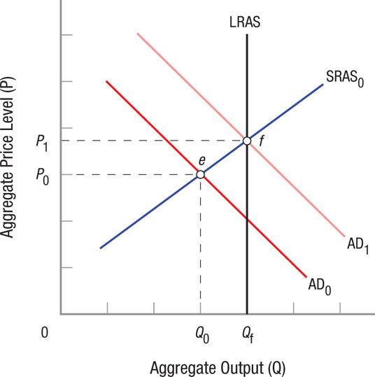
Figure 4 shows what happens when the economy is at full employment: An expansionary policy raises prices without producing any long-run improvement in real GDP. In this figure, the initial equilibrium is already at full employment (point e), therefore increasing aggregate demand moves the economy to a new output level above full employment (point a), thereby raising prices to P1. This higher output is only temporary, however, as workers and suppliers adjust their expectations to the higher price level, thus shifting short-run aggregate supply upward to SRAS2. Short-run aggregate supply declines because workers and other resource suppliers realize that the prices they are paying for products have risen; hence, they demand higher wages or prices for their services. This higher demand just pushes prices up further, until finally workers adjust their inflationary expectations and the economy settles into equilibrium at point b. At this point, the economy is again at full employment, but at a higher price level (P2) than before.
FIGURE 4
Expansionary Fiscal Policy at Full Employment When an economy is already at full employment, expansionary policies lead to no long-run improvement in real GDP. Beginning at full employment (point e), increasing aggregate demand moves the economy to an output level above full employment (point a). This higher output is only temporary, however, as workers and suppliers adjust their expectations to the higher price level (P1), thus shifting short-run aggregate supply left toward SRAS2. But this just pushes prices up further, until finally workers adjust their inflationary expectations, and the economy settles into a new long-run equilibrium at point b, where the economy is once again at full employment, but at a higher price level (P2).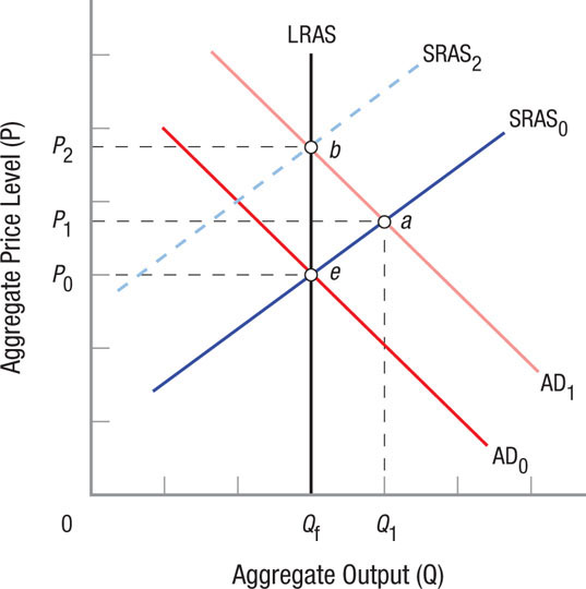
contractionary fiscal policy Involves increasing withdrawals from the economy by reducing government spending, transfer payments, or raising taxes to decrease aggregate demand to contract output and the economy.
When an economy moves to a point beyond full employment, as just described, economists say an inflationary spiral has set in. The explanation for this phenomenon was suggested earlier. Still, we can already see that one way to reduce such inflationary pressures is by a contractionary fiscal policy: reducing government spending, transfer payments, or raising taxes (increasing withdrawals from the economy). Figure 5 shows the result of contractionary policy. The economy is initially overheating at point e, with output above full employment. Contractionary policy reduces aggregate demand to AD1, bringing the economy back to full employment at price level P1 and output Qf.
FIGURE 5
Contractionary Fiscal Policy to Reduce Inflation In this figure, the economy is overheating at point e, with output above full employment. Contractionary policies reduce aggregate demand to AD1, bringing the economy back to full employment at price level P1. These policies prevent an inflationary spiral, but the fall in aggregate output leads to an increase in unemployment.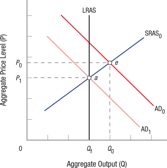
Exercising demand-side policy requires tradeoffs between increasing output at the expense of raising the price levels, or else lowering price levels by accepting a lower output. When recession threatens, the public is often happy to trade higher prices for greater employment and output. One would think the opposite would be true when an inflationary spiral loomed on the horizon. Politicians, however, are loath to support contractionary policies that control inflation by reducing aggregate demand, because high unemployment can cost politicians their jobs. As a result, the demand-side fiscal policy tools—government spending, transfer payments, and taxes—may remain unused. In these instances, politicians often look to the Federal Reserve to use its tools and influence to keep inflation in check. We will examine the Federal Reserve in later chapters.
FISCAL POLICY AND AGGREGATE DEMAND
- Demand-side fiscal policy involves using government spending, transfer payments, and taxes to change aggregate demand and equilibrium income, output, and the price level in the economy.
- In the short run, government spending raises income and output by the amount of spending times the multiplier. Tax reductions have a smaller impact on the economy than government spending because some of the reduction in taxes is added to saving and is therefore withdrawn from the economy.
- Expansionary fiscal policy involves increasing government spending, increasing transfer payments, or decreasing taxes.
- Contractionary fiscal policy involves decreasing government spending, decreasing transfer payments, or increasing taxes.
- When an economy is at full employment, expansionary fiscal policy may lead to greater output in the short term, but will ultimately just lead to higher prices in the longer term.
- Politicians tend to favor expansionary fiscal policy because it can bring with it increases in employment although with increasing inflation. Politicians tend to shun contractionary fiscal policy because it brings unemployment.
QUESTION: The 2009 $787 billion stimulus package cost roughly $2,500 per person or $10,000 for a family of four. The time required for the government to spend that sum on infrastructure projects (funding approvals, environmental clearances, and so on) means that the spending stretched over two to four years. Why didn’t Congress just send a $2,500 check to each woman, man, and child in America to speed up the impact on the economy?
Although the money would have hit the economy sooner, a significant portion of the proceeds would have been saved or used to pay existing bills, potentially limiting the stimulative impact of added spending. The other benefit of the infrastructure package is that by being spread out over several years, it won’t just be a big jolt to the economy that ends as fast as it began. Thus, the impact on employment and business planning was smoother.