Monetary Theories

In discussing the theories that justify the use of monetary policy, it is best to differentiate the long run from the short run. We will see that money has no effect on the real economy (such as employment and output) in the long run but can have an effect in the short run.

The Short Run Versus the Long Run: What’s the Difference?

One of the important concepts covered in Chapter 20 is the comparison between the short-run aggregate supply curve (SRAS) and the vertical long-run aggregate supply curve (LRAS). Recall that the LRAS curve is vertical because economic output is always fixed in the long run at the full employment output when wages and prices are flexible. Only factors that increase the productivity of inputs can shift the LRAS curve. The SRAS curve, however, is upward sloping because higher prices can cause temporary increases in output. This is due to sticky wages and prices.

We now build on the AD/AS model by explaining how changes in the money supply, which directly affect the aggregate demand curve, might change prices and output in the economy. The main determinant—you guessed it—depends on whether the aggregate supply curve is vertical (i.e., in the long run) or upward sloping (i.e., in the short run).

Let’s begin by looking at the long run, which is the analysis most commonly associated with the classical theory.

The Long Run: The Classical Theory

Classical economists focused on long-run adjustments in economic activity. In the long run, wages, prices, and interest rates are flexible, allowing the labor, product, and capital markets to adjust to keep the economy at full employment.

A product of the classical theory is the quantity theory of money, which is defined by the equation of exchange:

where M is the supply of money, V is the velocity of money (the average number of times per year a dollar is spent on goods and services), P is the price level, and Q is the economy’s real output level. Note that the right side of the equation—the aggregate price level times the level of output—is equal to nominal GDP.

In the long run, when the economy is at full employment, the implications for monetary policy are straightforward. Because velocity (V) is assumed to be fixed by existing monetary institutions (for example, the amount of cash you use on a monthly basis is generally consistent), and aggregate output (Q) is assumed to be fixed at full employment, any change in the money supply (M) will translate directly to a change in prices (P), or in other words, inflation.

Suppose you sell your grandma’s old LP records on eBay. Last month you listed five records for sale and sold them at an average winning bid of $20 each. Now suppose that this month a 10% increase in the money supply causes more people to want to buy records. If you again list only five records for sale, what will likely happen? There is more money to spend on the same amount of goods. Buyers might bid up the price to say, $22. In the end, prices rise in the exact proportion to the rise in the money supply. This is the essence of the classical theory—that increases in the money supply translate into an immediate and proportional rise in the aggregate price level with no change in real output (Q). As a result, monetary policy is ineffective.

Panel A of Figure 3 illustrates how the quantity theory works within an aggregate demand and supply model. The economy is initially in long-run equilibrium at point e with full employment output of $15 trillion and an initial money level of $2.0 trillion. Increasing the money supply to $2.2 trillion (a 10% increase) shifts aggregate demand upward to AD_($2.2T), resulting in a new equilibrium at point b where the aggregate price level increases to 110 (a 10% increase), yet real output remains constant at $15 trillion. This positive relationship between changes in the supply of money and inflation is evident in the plot shown in panel B, which shows the strong correlation between average monetary growth and inflation for 30 countries from 1972 to 2012. This suggests that any central bank that wants to avoid high inflation must avoid rapid growth of its money supply.

The Impact of a Change in the Money Supply in the Long Run: Theory and Evidence The quantity theory of money is shown using aggregate demand and aggregate supply. The economy is initially in equilibrium at point e. The long-run aggregate supply curve is vertical (long-run full employment at $15 trillion), while the aggregate demand curve reflects a money supply of $2.0 trillion. Increasing the money supply to $2.2 trillion (a 10% increase) shifts aggregate demand upward to AD_($2.2T), resulting in a new equilibrium at point b, where the aggregate price level rises by 10%, yet real output remains constant. The price level rise is equal to the percentage increase in the money supply. Monetary growth and inflation for thirty countries from 1972 to 2012 supports this theory.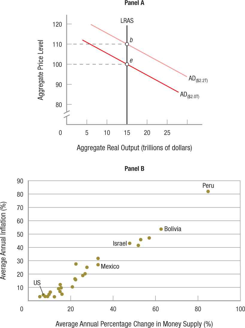

Quantity theory provides a good explanation of the long-run impact of monetary growth in the larger economy. But do people really catch on so quickly to money growth? Typically not. The realization that wages and prices can be “sticky” led economists to develop theories of how prices and output can change in the short run, leading to a SRAS curve that differs from a LRAS curve. The most notable theories include the Keynesian and monetarist models.

IRVING FISHER (1867–1947)

Irving Fisher was one of the ablest mathematical economists of the early 20th century. A staunch advocate of monetary reform, his theories influenced economists as different as John Maynard Keynes and Milton Friedman.

Born in upstate New York in 1867, Fisher studied mathematics, science, and philosophy at Yale University. In 1905, Fisher was in a phone booth in Grand Central Terminal in New York City when someone stole his briefcase, which contained his manuscript of The Nature of Capital and Income, one of the first economics books about the stock market. He rewrote the book in the next year, making copies of each chapter as it was finished and always closing the doors to phone booths after that.

Monetarists owe a great debt to Fisher’s next great book, The Purchasing Power of Money, in which he offered an “equation of exchange”: MV = PT (where T is the number of transactions taking place, or output). Classical economists have used variations of the formula to suggest that inflation is caused by increases in the money supply.

Fisher was prim and straight-laced, disciplined, and did not drink alcohol or coffee or tea, smoke, eat chocolate, or use pepper. His lack of humor and sometimes controversial economic beliefs (such as 100% bank reserves) led some to regard him as quite odd.

But among his many skills and interests, Fisher was a successful inventor and businessman. In 1925, he patented the “visible card index” system, an early version of the Rolodex, and earned a fortune. Unfortunately, within a few years he would lose everything in the stock market crash of 1929, an event that he famously failed to predict. His insistence of an imminent recovery during the early Depression years caused irreparable damage to a well-earned reputation as one of America’s greatest economists.

Sources: Justin Fox, The Myth of the Rational Market (New York: HarperCollins), 2009, p. 3; Robert Allen, Irving Fisher: A Biography (Cambridge, MA: Blackwell), 1993, p. 9.

Short-Run Effects of Monetary Policy

If the short-run effects of money were the same as in the long run, that would be the end of the story. In contrast to the long run, changes in the money supply can have an effect on the real economy in the short run, not just on the price level. To explain this, let’s start by returning to our earlier example to show how money supply growth can affect economic output.

Money Illusion and Sticky Wages and Prices Suppose you continue to sell your grandma’s records on eBay, listing five for sale each month. And every month, you notice that the average winning bids keep rising, first to $22, then to $25, then to $30, or even higher. This increase in the sales price makes you happy because you feel richer each month compared to the previous month. You think you are benefitting from the growing popularity of your grandma’s good taste in music.

How would you use your additional income? Most people would spend it by going out to eat more or buying more clothes. This extra spending (by you and everyone who feels richer) results in a temporary increase in economic output. But then you notice that the items you typically buy each month start increasing in price, so much so that despite earning more money, you end up buying about the same amount of goods as you did before. In other words, after prices caught up, you’re no better off than when you made only $20 per record. What you have discovered is that grandma’s records are not growing in popularity. Rather, growth in the money supply is causing an increase in all prices. You misperceived that you were wealthier when you really were not.

The example above illustrates the misperceptions in wealth that occur when the money supply grows, and is known as money illusion. But money illusion is not the only distinguishing factor between the short run and the long run. Another short-run effect is that wages and prices tend to react slowly to changes in the economy. Most workers’ wages do not change with every paycheck; similarly, the prices of many goods and services we buy do not change every day. This delayed reaction in wages and prices to economic conditions makes them sticky. This is not the first time we have studied the effects of sticky wages and sticky prices—we studied them previously when explaining why the SRAS curve slopes upward. But now we look at how an upward sloping SRAS curve can make monetary policy effective in the short run by looking at two opposing views on the effectiveness of monetary policy in the short run.

Keynesian Model Developed by John Maynard Keynes during the Great Depression of the 1930s, Keynesian analysis has had a profound effect on policymakers and economists that continues today. According to Keynesian theory, an increase in the money supply leads more people to buy interest-earning assets (bonds), causing the price of bonds to rise and the interest rate to fall. Lower interest rates should normally lead to an increase in investment that increases aggregate demand, which increases income, output, and employment.

However, Keynesians believed that this outcome occurs only when the economy is healthy. During times of recession, people become fearful and don’t buy as much, leading to massive excess capacity for businesses. Reducing interest rates might not lead to greater investment, because firms are unable to sell what they were currently producing, and therefore would be reluctant to invest more.

Further, when interest rates fall to very low levels, Keynes argued that people simply hoard money because it’s not worth holding bonds that pay so little interest. Keynes referred to this phenomenon as the liquidity trap. In a liquidity trap, an increase in the money supply does not result in a decrease in interest rates; thus there is no change in investment, and consequently no change in income or output. Monetary policy is totally ineffective. This was one reason Keynes argued that fiscal policy, especially government spending, was needed to get the economy out of the Depression.

Monetarist Model Milton Friedman challenged the Keynesian view by arguing that government spending inherent to fiscal policy must be financed either by increased taxation and/or increased borrowing. His monetarist theory states that higher taxation means consumers and firms have less money to consume and invest, while increased borrowing leads to higher interest rates, which also reduces consumption and investment. Thus, monetarists believe that the crowding out effect makes fiscal policy ineffective.

Friedman pioneered the notion that consumption is not only based on income, but also on wealth, an idea he referred to as the permanent income hypothesis.

NOBEL PRIZE MILTON FRIEDMAN (1912–2006)

Milton Friedman may be the best-known economist of the latter half of the 20th century. During the 1980s, his advocacy of free market economics and “monetarist” theories had a dramatic impact on policymakers, notably President Ronald Reagan and British Prime Minister Margaret Thatcher. His book, A Monetary History of the United States, 1867–1960, co-authored with Anna Schwartz, is considered a modern classic of economics.

Born in 1912 in Brooklyn, New York, to poor immigrant parents, Friedman was awarded a scholarship to Rutgers University but paid for his additional expenses by waiting on tables and clerking in a store. He eventually went on to graduate school at the University of Chicago to study economics, and then to Columbia University.

In 1946, he accepted a professorship at the University of Chicago where he delved into the role of money in business cycles. In 1950, Friedman worked in Paris for the Marshall Plan, studying a precursor to the Common Market. He came to believe in the importance of flexible exchange rates between members of the European community.

Friedman’s views were explicitly counter to the Keynesian belief in a range of activist government policies to stabilize the economy. Friedman emphasized the importance of monetary policy in determining the level of economic activity, and advocated a consistent policy of steady growth in the money supply to encourage stability and economic growth.

Friedman was awarded the Nobel Prize in Economics in 1976 for his work on monetary theories and also for his concept of “permanent income,” the idea that people based their savings habits on the typical amount they earn instead of on increases or decreases they may view as temporary.

With Friedman’s approach, when the money supply increases, interest rates fall, and individuals rebalance their asset portfolios by exchanging money for other assets, not only bonds—for example, real estate and consumer durables such as cars and recreational equipment. Therefore, falling interest rates will lead to higher investment and/or consumption. This leads to an increase in aggregate demand and ultimately an increase in income, output, and/or the price level.

Therefore, monetarists believe that monetary policy can be effective in the short run. But, like classical economists, monetarists believe that an increase in money will ultimately increase prices in the long run. As Milton Friedman famously remarked: “Inflation is always and everywhere a monetary phenomenon.”

Figure 4 illustrates the monetarist approach that a change in output will occur only in the short run. The economy is initially in long-run equilibrium at point e, with output at $15 trillion and a price level of 100. A 10% increase in the money supply from $2.0 trillion to $2.2 trillion shifts the aggregate demand curve from AD₀ to AD₁, initially raising output to $16 trillion and the aggregate price level to 104 (point b). Over time, as prices adjust, the SRAS curve will shift left and the economy will move back to its full employment output ($15 trillion), raising prices in the long run by 10% to 110 (point c).

Monetarist Theory on Money Supply Monetarists argue that a change in output will last only for the short run; in the long run, the economy will move back to full employment. The economy begins in equilibrium at point e. An increase in the money supply of 10% shifts the aggregate demand curve from AD₀ to AD₁, resulting in higher short-run output, $16 trillion, and a higher price level (point b). Over time, the economy will move back to full employment ($15 trillion), increasing the price level in the long run to 110 (a 10% increase). The long-run aggregate supply curve is therefore vertical at full employment output ($15 trillion).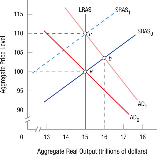

Summary of the Effectiveness of Monetary Policy

Let’s summarize the theories of the effectiveness of monetary policy.

Long Run: Changes in the money supply show up directly as increases in the price level because both velocity and output are considered fixed in the equation of exchange (M × V = P × Q). Because classical economists focused on the long run, they saw no use for monetary policy.

Short Run: Keynes believed that when the economy is well below full employment, monetary policy is ineffective because investment is more influenced by business expectations about the economy than interest rates. Further, Keynes suggested that once interest rates get very low, monetary policy might confront a “liquidity trap,” where money is just hoarded. Thus, Keynesians favor fiscal policy to move the economy toward full employment.

Monetarists, on the other hand, do see a role for monetary policy. In the short run, changes in the money supply reduce interest rates, which in turn stimulate both investment and consumption. Consumer spending is related to wealth (not just income), and changes in interest rates induce portfolio adjustments that alter consumer spending for durable goods.

A summary of the three theories is provided in Table 1.

Monetary Policy and Economic Shocks

Our discussion thus far suggests that the Fed’s approach to monetary policy should be based on both short- and long-run considerations. Low inflation represents a reasonable long-run goal, while income and output are more appropriate for the shorter term.

Economists generally agree that, in the long run, the Fed should focus on price stability because low rates of inflation have been shown to create the best environment for long-run economic growth.

We have seen from the equation of exchange that, in the long run, aggregate supply is vertical and fixed at full employment, and changes in the supply of money result directly in changes in the price level.

But in the short run, demand and supply shocks to the economy may require differing approaches to monetary policy. The direction of monetary policy and its extent depend on whether it focuses on the price level or income and output, and whether the shock to the economy comes from the demand or the supply side.

Demand Shocks Demand shocks to the economy can come from reductions in consumer demand, investment, government spending, or exports, or from an increase in imports. For example, the economy faced a demand shock in 2008 when households, fearing unemployment after the housing bubble burst, increased saving and reduced spending. Let’s consider an economy that is initially in full employment equilibrium at point e in panel A of Figure 5. A demand shock then reduces aggregate demand to AD₁. At the new equilibrium (point a), the price level and output both fall.

Demand Shocks, Supply Shocks, and Monetary Policy Monetary policy can be effective in counteracting a demand shock. In panel A, the economy begins in full employment equilibrium at point e and then a demand shock reduces aggregate demand to AD₁, resulting in a new equilibrium (point a). Expansionary monetary policy will shift aggregate demand back to AD₀. This policy restores output back to full employment ($15 trillion), while restoring prices to their original level (100). Monetary policy is less effective in counteracting a supply shock. In panel B, a negative supply shock shifts short-run aggregate supply from SRAS₀ to SRAS₁. The new equilibrium (point a) is at a higher price level, 105, and lower output, $14 trillion, a doubly negative result. The Fed could use expansionary monetary policy to shift AD₀ to AD₁; this would restore the economy to full employment output of $15 trillion (point b), but at an even higher price level (110). Alternatively, the Fed could focus on price level stability, using contractionary monetary policy to shift aggregate demand to AD₂, but this would further deepen the recession by pushing output down to $13 trillion (point c).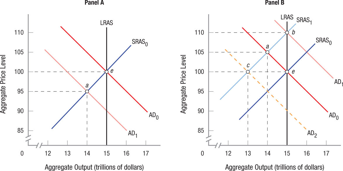

An expansionary monetary policy will increase the money supply, lower interest rates, and thereby shift aggregate demand back to AD₀, restoring employment and output to full employment. In this case, targeting either a stable price level (100) or the original income and output level ($15 trillion) will bring the economy back to the same point of equilibrium, point e, where both targets are reached.

A positive demand shock produces a corresponding, though opposite, result. The positive demand shock will jolt output and the price level upward. Contractionary monetary policy will reduce both of them, restoring the economy to its original equilibrium.

For demand shocks, therefore, no conflict arises between the twin goals of monetary policy. Not only is the objective of full employment compatible with the objective of stable prices, but by targeting either one of these objectives, the Fed takes steps that work to bring about the other.

Supply Shocks Supply shocks can hit the economy for many reasons, including changes in resource costs such as a rise in oil prices, changes in inflationary expectations, or changes in technology. Looking at panel B of Figure 5, let us again consider an economy initially in full employment equilibrium at point e. Assume that a negative shock to the economy, say, an oil price spike, shifts short-run aggregate supply from SRAS₀ to SRAS₁. The new equilibrium (point a) occurs at a higher price level (105) and a lower output of $14 trillion.

This doubly negative result means that a supply shock is very difficult to counter. The Fed could use expansionary monetary policy to shift AD₀ to AD₁; this would restore the economy to full employment output of $15 trillion (point b), but at an even higher price level (110). Alternatively, the Fed could focus on price level stability, using contractionary monetary policy to shift aggregate demand to AD₂, but this would further deepen the recession by pushing output down to $13 trillion (point c).

For a negative supply shock, not only has price level stability worsened, but so has output and income. Contrast this with the situation earlier, when a demand shock worsened the economy for one of its targets, but improved it for the other. Supply shocks are difficult to counteract because of their doubly negative results.

Implications for Short-Run Monetary Policy There is general agreement among economists that monetary policy should focus on price stability in the long run, while focusing on output or income in the short run. When a demand shock strikes, following this short-run policy course has the same effect as using price stability as the goal. When a supply shock occurs, however, targeting nominal income or output is preferable, because it permits the Fed to spread the shock’s impact between income and output losses and price level increases. By increasing aggregate demand, the economy will suffer some added increase in the price level, but output will rise, reducing the severity of any recession. The Fed will probably not try to push the economy back to full employment (from point a to point b in the right panel in Figure 5) immediately, because this action would result in much higher inflation. Moving the economy back to full employment is typically spread over several periods.