Market Equilibrium
equilibrium Market forces are in balance when the quantities demanded by consumers just equal the quantities supplied by producers.
equilibrium price Market equilibrium price is the price that results when quantity demanded is just equal to quantity supplied.
equilibrium quantity Market equilibrium quantity is the output that results when quantity demanded is just equal to quantity supplied.
Supply and demand together determine the prices and quantities of goods bought and sold. Neither factor alone is sufficient to determine price and quantity. It is through their interaction that supply and demand do their work, just as two blades of a scissors are required to cut paper.
A market will determine the price at which the quantity of a product demanded is equal to the quantity supplied. At this price, the market is said to be cleared or to be in equilibrium, meaning that the amount of the product that consumers are willing and able to purchase is matched exactly by the amount that producers are willing and able to sell. This is the equilibrium price and the equilibrium quantity. The equilibrium price is also called the market-clearing price.
Figure 9 puts together Figures 2 and 5, showing the market supply and demand for computer games. It illustrates how supply and demand interact to determine equilibrium price and quantity. Clearly, the quantities demanded and supplied equal one another only where the supply and demand curves cross, at point e. Alternatively, you can see this in the table that is part of the figure: Quantity demanded and quantity supplied are the same at only one particular point. At $60 per game, sellers are willing to provide exactly the same quantity as consumers would like to purchase. Hence, at this price, the market clears, since buyers and sellers both want to transact the same number of units.
FIGURE 9
Equilibrium Price and Quantity of Computer Games Market equilibrium is achieved when quantity demanded and quantity supplied are equal. In this graph, that equilibrium occurs at point e, at an equilibrium price of $60 and an equilibrium output of 30. If the market price is above equilibrium ($80), a surplus of 20 computer games will result (b − a), and market forces would drive the price back down to $60. When the market price is too low ($40), a shortage of 20 computer games will result (d − c), and businesses will raise the offering prices until equilibrium is again restored.
surplus Occurs when the price is above market equilibrium, and quantity supplied exceeds quantity demanded.
The beauty of a market is that it automatically works to establish the equilibrium price and quantity, without any guidance from anyone. To see how this happens, let us assume that computer games are initially priced at $80, a price above their equilibrium price. As we can see by comparing points a and b, sellers are willing to supply more games at this price than consumers are willing to buy. Economists characterize such a situation as one of excess supply, or surplus. In this case, at $80, sellers supply 40 games to the market (point b), yet buyers want to purchase only 20 (point a). This leaves an excess of 20 games overhanging the market; these unsold games ultimately become surplus inventories.
Here is where the market kicks in to restore equilibrium. As inventories rise, most firms cut production. Some firms, moreover, start reducing their prices to increase sales. Other firms must then cut their own prices to remain competitive. This process continues, with firms cutting their prices and production, until most firms have managed to exhaust their surplus inventories. This happens when prices reach $60 and quantity supplied equals 30, because consumers are once again willing to buy up the entire quantity supplied at this price, and the market is restored to equilibrium.
shortage Occurs when the price is below market equilibrium, and quantity demanded exceeds quantity supplied.
In general, therefore, when prices are set too high, surpluses result, which drive prices back down to their equilibrium levels. If, conversely, a price is initially set too low, say at $40, a shortage results. In this case, buyers want to purchase 40 games (point d), but sellers are only providing 20 (point c), creating a shortage of 20 games. Because consumers are willing to pay more than $40 to obtain the few games available on the market, they will start bidding up the price of computer games. Sensing an opportunity to make some money, firms will start raising their prices and increasing production once again until equilibrium is restored. Hence, in general, excess demand causes firms to raise prices and increase production.
When there is a shortage in a market, economists speak of a tight market or a seller’s market. Under these conditions, producers have no difficulty selling off all their output. When a surplus of goods floods the market, this gives rise to a buyer’s market, because buyers can buy all the goods they want at attractive prices.
We have now seen how changing prices naturally works to clear up shortages and surpluses, thereby returning markets to equilibrium. Some markets, once disturbed, will return to equilibrium quickly. Examples include the stock, bond, and money markets, where trading is nearly instantaneous and extensive information abounds. Other markets react very slowly. Consider the labor market, for instance. When workers lose their jobs due to a plant closing, most will search for new jobs that pay at least as much as that at their previous jobs. Some will be successful, while others might struggle, having to settle for a lower paying position after a long job search. Similarly, real estate markets can be slow to adjust because sellers will often refuse to accept a price below what they are asking, until the lack of sales over time convinces sellers to adjust the price downward.
ALFRED MARSHALL(1842–1924)
British economist Alfred Marshall is considered the father of the modern theory of supply and demand—that price and output are determined by both supply and demand. He noted that the two go together like the blades of a scissors that cross at equilibrium. He assumed that changes in quantity demanded were only affected by changes in price, and that all other factors remained constant. Marshall also is credited with developing the ideas of the laws of demand and supply, and the concepts of consumer surplus and producer surplus—concepts we will study in the next chapter.
With financial help from this uncle, Marshall attended St. John’s College, Cambridge, to study mathematics and physics. However after long walks through the poorest sections of several European cities and seeing their horrible conditions, he decided to focus his attention on political economy.
In 1890, he published Principles of Economics. In it he introduced many new ideas, though he would never boast about them as being novel. In hopes of appealing to the general public, Marshall buried his diagrams in footnotes. And, although he is credited with many economic theories, he would always clarify them with various exceptions and qualifications. He expected future economists to flesh out his ideas.
Above all, Marshall loved teaching and his students. His lectures were known to never be orderly or systematic because he tried to get students to think with him and ultimately think for themselves. At one point near the turn of the twentieth century, essentially all of the leading economists in England had been his students. More than anyone else, Marshall is given credit for establishing economics as a discipline of study. He died in 1924.
Sources: E. Ray Canterbery A Brief History of Economics: Artful Approaches to the Dismal Science (Hackensack, New Jersey: World Scientific), 2001; Robert Skidelsky, John Maynard Keynes: Volume 2, The Economist as Saviour 1920–1937 (New York: Penguin Press), 1992; and John Maynard Keynes, Essays in Biography (New York: Norton), 1951.
These automatic market adjustments can make some buyers and sellers feel uncomfortable: It seems as if prices and quantities are being set by forces beyond anyone’s control. In fact, this phenomenon is precisely what makes market economies function so efficiently. Without anyone needing to be in control, prices and quantities naturally gravitate toward equilibrium levels. Adam Smith was so impressed by the workings of the market that he suggested that it is almost as if an “invisible hand” guides the market to equilibrium.
Given the self-correcting nature of the market, long-term shortages or surpluses are almost always the result of government intervention, as we will see in the next chapter. First, however, we turn to a discussion of how the market responds to changes in supply and demand, or to shifts of the supply and demand curves.
Moving to a New Equilibrium: Changes in Supply and Demand
Once a market is in equilibrium and the forces of supply and demand balance one another out, the market will remain there unless an external factor changes. But when the supply curve or demand curve shifts (some determinant changes), equilibrium also shifts, resulting in a new equilibrium price and/or output. The ability to predict new equilibrium points is one of the most useful aspects of supply and demand analysis.
Predicting the New Equilibrium When One Curve Shifts When only supply or only demand changes, the change in equilibrium price and equilibrium output can be predicted. We begin with changes in supply.
Changes in Supply Figure 10 shows what happens when supply changes. Equilibrium initially is at point e, with equilibrium price and quantity at $9 and 30, respectively. But let us assume that a rise in wages or the bankruptcy of a key business in the market (the number of sellers falls) causes a decrease in supply. When supply declines (the supply curve shifts from S0 to S2), equilibrium price rises to $12, while equilibrium output falls to 20 (point a).
FIGURE 10
Equilibrium Price, Output, and Shifts in Supply When supply alone shifts, the effects on both equilibrium price and output can be predicted. When supply grows (S0 to S1), equilibrium price will fall and output will rise. When supply declines (S0 to S2), the opposite happens: Equilibrium price will rise and output will fall.
If, on the other hand, supply increases (the supply curve shifts from S0 to S1), equilibrium price falls to $6, while equilibrium output rises to 40 (point b). This is what has happened in the electronics industry: Falling production costs have resulted in more electronic products being sold at lower prices.
We can predict how equilibrium price and quantity will change when supply changes. When supply increases, equilibrium price will fall and output will rise; when supply decreases, equilibrium price will rise and output will fall.
Changes in Demand The effects of demand changes are shown in Figure 11. Again, equilibrium is initially at point e, with equilibrium price and quantity at $9 and 30, respectively. But let us assume that the economy then enters a recession and incomes sink, or perhaps the price of some complementary good soars; in either case, demand falls. As demand decreases (the demand curve shifts from D0 to D2), equilibrium price falls to $6, while equilibrium output falls to 20 (point a).
FIGURE 11
Equilibrium Price, Output, and Shifts in Demand When demand alone changes, the effects on both equilibrium price and output can again be determined. When demand grows (D0 to D1), both price and output rise. Conversely, when demand falls (D0 to D2), both price and output fall.
During the same recession just described, the demand for inferior goods (beans and bologna) will rise, as falling incomes force people to switch to less expensive substitutes. For these products, as demand increases (shift ing the demand curve from D0 to D1), equilibrium price rises to $12, and equilibrium output grows to 40 (point b).
Like changes in supply, we can predict how equilibrium price and quantity will change when demand changes. When demand increases, both equilibrium price and output will rise; when demand decreases, both equilibrium price and output will fall.
Two-Buck Chuck: Will People Drink $2-a-Bottle Wine?
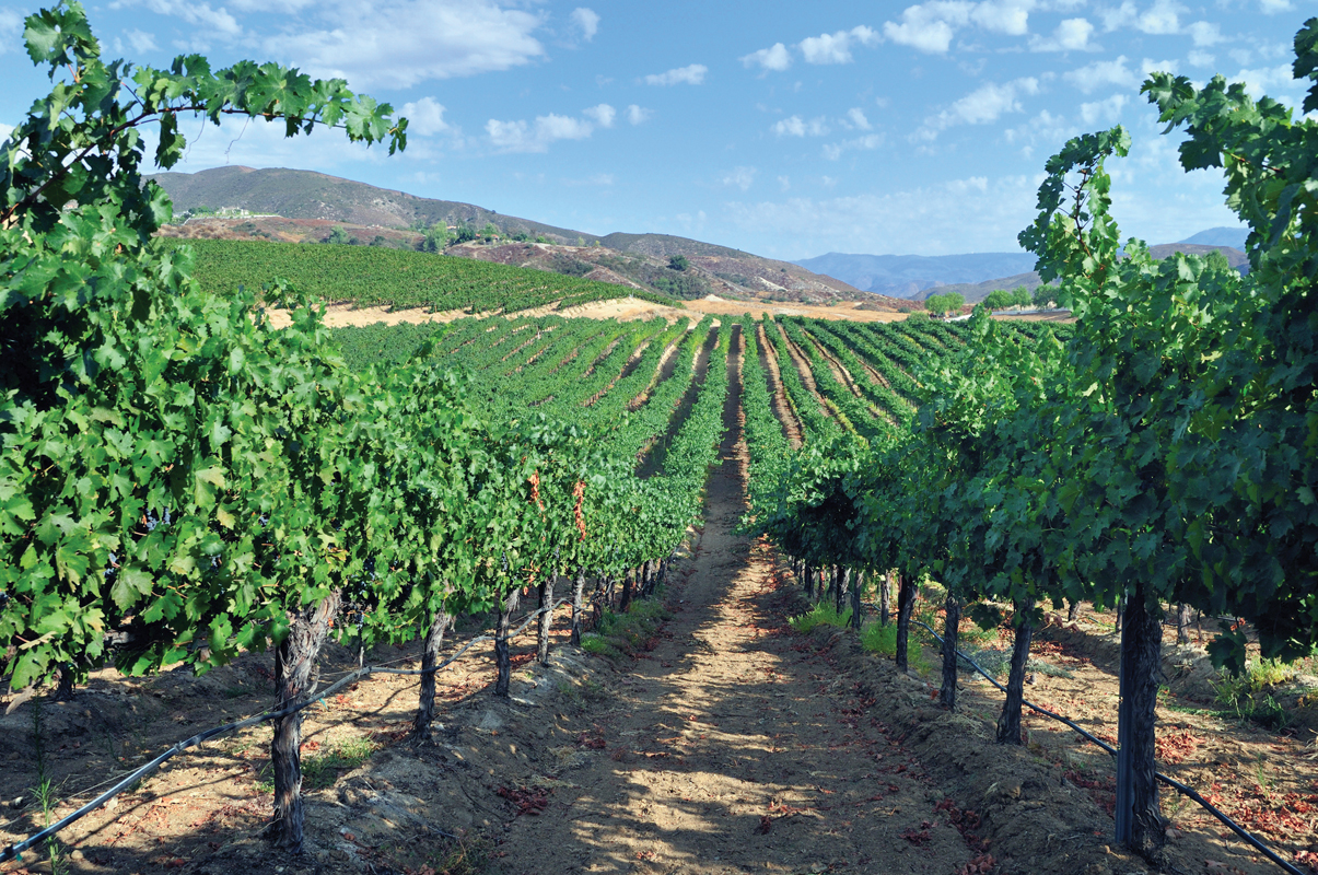
The great California wines of the 1990s put California vineyards on the map. Demand, prices, and exports grew rapidly. Overplanting of new grapevines was a result. When driving along Interstate 5 or Highway 101 north of Los Angeles, one can see vineyards extending for miles, and most were planted in the mid- to late 1990s. The 2001 recession reduced the demand for California wine, and a rising dollar made imported wine relatively cheaper. The result was a sharp drop in demand for California wine and a huge surplus of grapes.
Bronco Wine Company president Fred Franzia made an exclusive deal with Trader Joe’s, an unusual supermarket that features exotic food and wine products. He bought the excess grapes at distressed prices, and in his company’s modern plant produced inexpensive wines—chardonnay, merlot, cabernet sauvignon, shiraz, and sauvignon blanc—under the Charles Shaw label. Consumers flocked to Trader Joe’s for wine costing $1.99 a bottle and literally hauled cases of wine out by the carload. In less than a decade, 400 million bottles of Two-Buck Chuck, as it is known, have been sold. This is not rotgut: The 2002 shiraz beat out 2,300 other wines to win a double gold medal at the 28th Annual International Eastern Wine Competition in 2004. Still, to many Napa Valley vintners it is known as Two-Buck Upchuck.
Two-Buck Chuck was such a hit that other supermarkets were forced to offer their own discount wines. This good, low-priced wine has had the effect of opening up markets. People who previously avoided wine because of the cost have begun drinking more. However, the influence of Two-Buck Chuck, which sold 60 million bottles in 2012, may be waning. In January 2013, Trader Joe’s announced an increase in the price of the Two-Buck Chuck from $1.99 to $2.49 due to a poor grape harvest that raised the cost of producing the wine. Although the new price is still a bargain, the product that changed the wine industry may soon need another name.
Predicting the New Equilibrium When Both Curves Shift When both supply and demand change, things get tricky. We can predict what will happen with price in some cases and output in other cases, but not what will happen with both.
Figure 12 portrays an increase in both demand and supply. Consider the market for corn. Suppose that an increase in corn-based ethanol production causes demand for corn to increase. Meanwhile, suppose that bioengineering results in a new corn hybrid that uses less fertilizer and generates 50% higher yields, causing supply to also increase. When demand increases from D0 to D1 and supply increases from S0 to S1, output grows to Q1 as shown in the left panel.
FIGURE 12
Increase in Supply, Increase in Demand, and Equilibrium When both demand and supply increase, output will clearly rise, but what happens to the new equilibrium price is uncertain. If demand grows relatively more than supply, price will rise, but if supply grows relatively more than demand, price will fall.
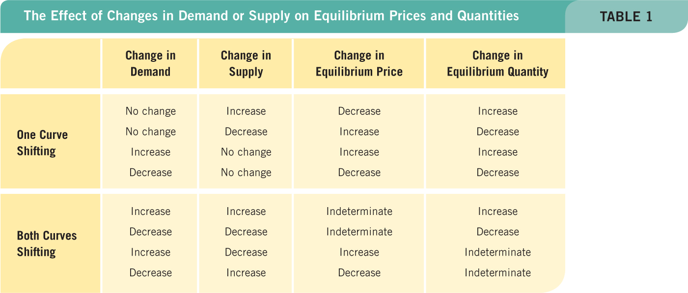
But what happens to the price of corn is not so clear. If demand and supply grow the same, output increases but price remains at P0 (also captured in the middle panel to the right). If demand grows relatively more than supply, the new equilibrium price will be higher (top panel on the right). Conversely, if demand grows relatively less than supply, the new equilibrium price will be lower (bottom panel on the right). Figure 12 is just one of the four possibilities when both supply and demand change. The other three possibilities are shown in Table 1 along with the four possibilities when just one curve shifts. When only one curve shifts, the direction of change in equilibrium price and quantity is certain. But when both curves shift, the direction of change in either the equilibrium price or quantity will be indeterminate.
MARKET EQUILIBRIUM
- Together, supply and demand determine market equilibrium, which occurs when the quantity supplied exactly equals quantity demanded.
- The equilibrium price is also called the market-clearing price.
- When quantity demanded exceeds quantity supplied, a shortage occurs and prices are bid up toward equilibrium. When quantity supplied exceeds quantity demanded, a surplus occurs and prices are pushed down toward equilibrium.
- When supply and demand change, equilibrium price and output change.
- When only one curve shifts, the resulting changes in equilibrium price and quantity can be predicted.
- When both curves shift, we can predict the change in equilibrium price in some cases or the change in equilibrium quantity in others, but never both. We have to determine the relative magnitudes of the shifts before we can predict both equilibrium price and quantity.
QUESTIONS: As China and India (both with huge populations and rapidly growing economies) continue to develop, what do you think will happen to their demand for energy, and specifically oil? What will suppliers of oil do in the face of this demand? Will this have an impact on world energy (oil) prices? What sort of policies or events could alter your forecast about the future price of oil?
Demand for both energy and oil will increase. Suppliers of oil will attempt to move up their supply curve and provide more to the market. Because all of the easy (cheap) oil has already been found, costs to add to supplies will rise, and oil prices will gradually rise; in the longer term, alternatives will become more attractive, keeping oil prices from rising too rapidly.