Section 1: Aggregate Demand

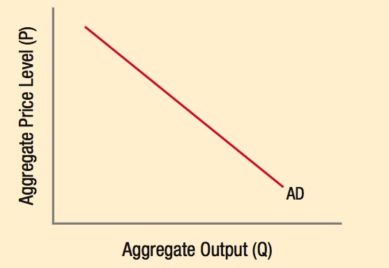
The aggregate demand curve shows the quantity of goods and services (real GDP) demanded at different price levels.

The determinants of aggregate demand include the components of aggregate spending:

1. Consumption spending
2. Investment spending
3. Government spending
4. Net exports

Changing any one of these aggregates will shift the aggregate demand curve.

The aggregate demand curve is downward sloping for three main reasons:

• Wealth effect: When price levels rise, the purchasing power of money saved falls.
• Export effect: Rising price levels cause domestic goods to be more expensive in the global marketplace, resulting in fewer purchases by foreign consumers.
• Interest rate effect: When price levels rise, people need more money to carry out transactions. The added demand for money drives up interest rates, causing investment spending to fall.

The housing market recovery has resulted in a boost to aggregate demand.

Section 2: Aggregate Supply

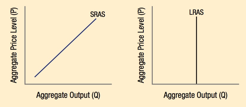
The aggregate supply curve shows the real GDP firms will produce at varying price levels.

In the short run, aggregate supply is upward-sloping (SRAS).

In the long run, aggregate supply is vertical (LRAS).

In the short run, prices and wages are sticky (think of menu prices staying the same for a period of time). Therefore firms respond by increasing output when prices rise.

In the long run, prices and wages adjust, therefore output is not affected by the price level.

Factors that shift the SRAS curve:

• Input prices
• Productivity
• Taxes and regulation
• Market power of firms
• Expectations

Factors that shift the LRAS curve:

• Increase in technology
• Greater human capital
• Trade
• Innovation and R&D

Electronic toll collection booths save time and reduce transportation costs to firms, leading to an increase in short-run aggregate supply and potentially long-run aggregate supply.

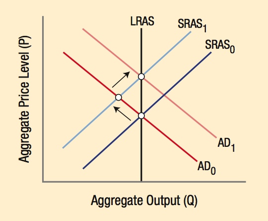
Section 3: Macroeconomic Equilibrium

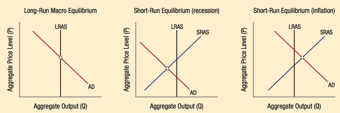
A long-run macroeconomic equilibrium occurs at the intersection of the LRAS and AD curves, at full employment.

A short-run macroeconomic equilibrium occurs at the intersection of the SRAS and AD curves. Short-run equilibrium can occur below full employment (recession) or above full employment (inflationary pressure).

The spending multiplier exists because new spending generates income that results in more spending and income, based on the marginal propensities to consume and save.

Multiplier Example: MPC = 0.80 and MPS = 0.20

Round 1: $100 in new spending = $100 in new income

Round 2: $80 is spent and $20 is saved ($80 in new income)

Round 3: $64 is spent and $16 is saved

Round 4: $51.20 is spent and $12.80 is saved

Round 5: $40.96 is spent and $10.24 is saved

Round 6: $32.76 is spent and $8.20 is saved

…

Round n: $0.01 is spent and $0.00 is saved

Total effect of $100 in spending = $500 in spending and $100 in savings

Multiplier = 1/(1 − MPC) = 1/(1 − 0.80) = 5

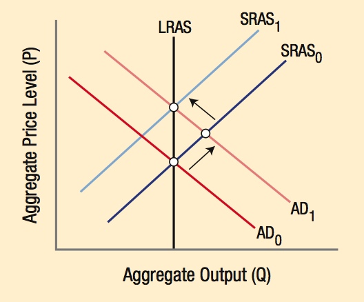
Demand-pull inflation occurs when aggregate demand expands so much that equilibrium output exceeds full employment output. Temporarily, the economy can expand beyond full employment as workers incur overtime and more workers are added. But as wages rise, the economy will move to a new equilibrium, where prices are permanently higher.

Cost-push inflation occurs when a supply shock hits the economy, shifting the SRAS curve to the left. Cost-push inflation makes using policies to expand aggregate demand to restore full employment difficult because of the additional inflationary pressures added to the economy.