Ceteris Paribus, Simple Equations, and Shifting Curves
Hold on while we beat this GPA and studying example into the ground. Inevitably, when we simplify analysis to develop a graph or model, important factors or influences must be controlled. We do not ignore them, we hold them constant. These are known as ceteris paribus assumptions.
Ceteris Paribus: All Else Equal
By ceteris paribus we mean other things being equal or all other relevant factors, elements, or influences are held constant. When economists define your demand for a product, they want to know how much or how many units you will buy at different prices. For example, to determine how many DVDs you will buy at various prices (your demand for DVDs), we hold your income and the price of movie tickets and online movie downloads constant. If your income suddenly jumped, you would be willing to buy more DVDs at all prices, but this is a whole new demand curve. Ceteris paribus assumptions are a way to simplify analysis; then the analysis can be extended to include those factors held constant, as we will see next.
Simple Linear Equations
Simple linear equations can be expressed as: Y = a + bX. This is read as, Y equals a plus b times X, where Y is the variable plotted on the y axis and a is a constant (unchanging), and b is a different constant that is multiplied by X, the value on the x axis. The formula for our studying and GPA example introduced in Figure APX-6 is shown in Figure APX-10.
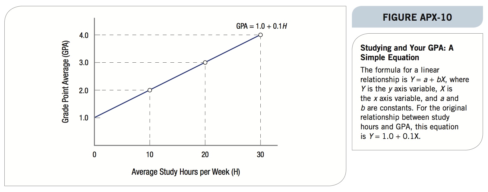
The constant a is known as the vertical intercept because it is the value of GPA when study hours (X) is zero, and therefore it cuts (intercepts) the vertical axis at the value of 1.0 (D average). Now each time you study another hour on average, your GPA rises by 0.1, so the constant b (the slope of the line) is equal to 0.1. Letting H represent hours of studying, the final equation is: GPA = 1.0 + 0.1H. You start with a D average without studying and as your hours of studying increase, your GPA goes up by 0.1 times the hours of studying. If we plug in 20 hours of studying into the equation, the answer is a GPA of 3.0 [1.0 + (0.1 × 20) = 1.0 + 2.0 = 3.0].
25
Shifting Curves
Now let’s introduce a couple of factors that we have been holding constant (the ceteris paribus assumption). These two elements are tutoring and partying. So, our new equation now becomes GPA = 1.0 + 0.1H + Z, where Z is our variable indicating whether you have a tutor or whether you are excessively partying. When you have a tutor, Z = 1, and when you party too much, Z = −1. Tutoring adds to the productivity of your studying (hence Z = 1), while excessive late-night partying reduces the effectiveness of studying because you are always tired (hence Z = −1). Figure APX-11 shows the impact of adding these factors to the original relationship.
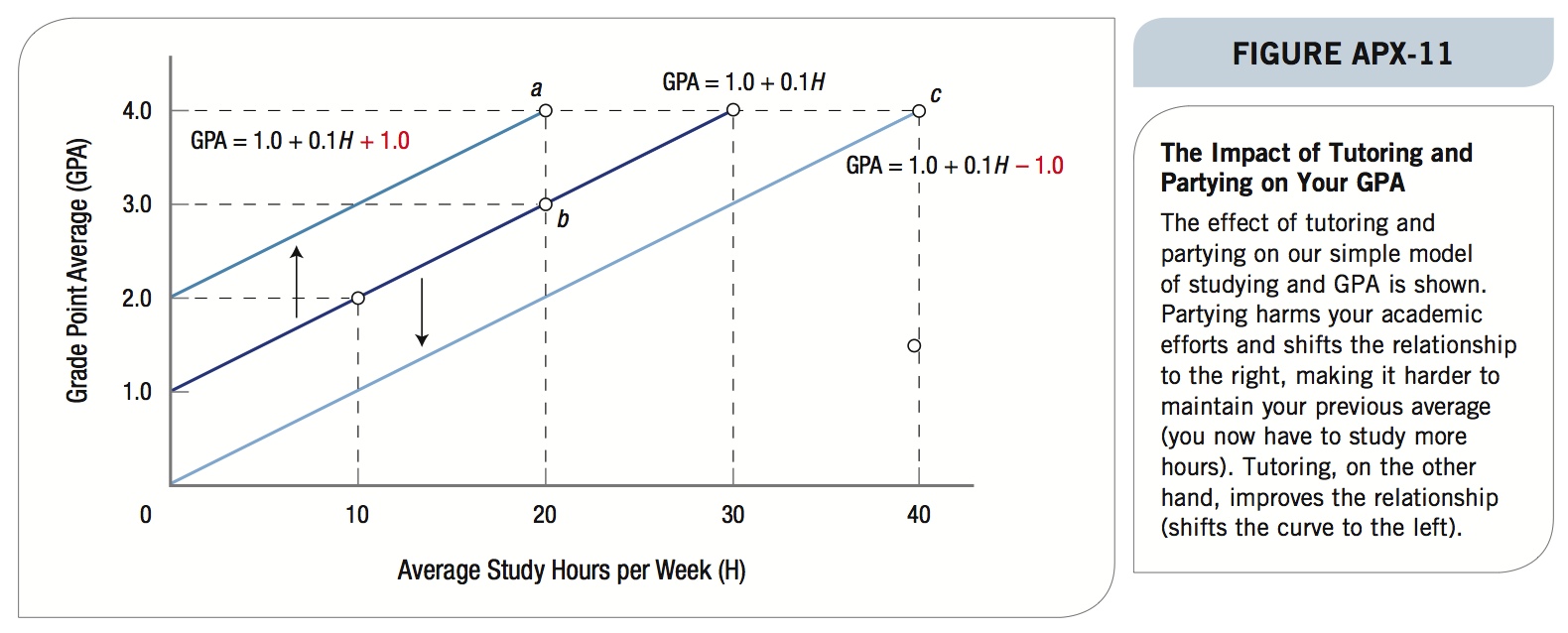
With tutoring, your GPA-studying curve has moved upward and to the left. Now, because Z = 1, you begin with a C average (2.0), and with just 20 hours of studying (because of tutoring) you can reach a 4.0 GPA (point a). Alternatively, when you don’t have tutoring and you party every night, your GPA–studying relationship has worsened (shifted downward and to the right). Now you must study 40 hours (point c) to accomplish a 4.0 GPA. Note that you begin with failing grades.
26
The important point here is that we can simplify relationships between different variables and use a simple graph or equation to represent a model of behavior. In doing so, we often have to hold some things constant. When we allow those factors to change, the original relationship is now changed and often results in a shift in the curves. You will see this technique applied over and over as you study economics this term.