AGGREGATE EXPENDITURES
aggregate expenditures Consist of consumer spending, business investment spending, government spending, and net foreign spending (exports minus imports): GDP = C + I + G + (X − M).
Recall that when we discussed measuring gross domestic product (GDP), we concluded that it could be computed by adding up either all spending or all income in the economy. We saw that the expenditures side consists of consumer spending, business investment spending, government spending, and net foreign spending (exports minus imports). Thus, aggregate expenditures are equal to
GDP = AE = C + I + G + (X – M)
Some Simplifying Assumptions
In this chapter, we first will focus on a simple model of the private economy that includes only consumers and businesses. Later in the chapter, we will incorporate government spending, taxes, and the foreign sector into our analysis. Second, we will assume that all saving is personal saving as opposed to national saving, which includes business saving and government saving. Third, because Keynes was modeling a depression economy, we follow him in assuming that there is considerable slack in the economy, much like the economy during and in the years following the 2007–
Consumption and Saving
consumption Spending by individuals and households on both durable goods (e.g., autos, appliances, and electronic equipment) and nondurable goods (e.g., food, clothing, and entertainment).
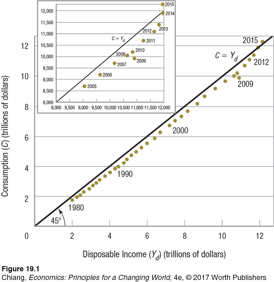
Personal consumption expenditures (C) represent about 68% of GDP, and for this reason consumption is a major ingredient in our model. Figure 1 shows personal consumption expenditures for the years since 1980. Notice how closely consumption parallels disposable income.
saving The difference between income and consumption; the amount of disposable income not spent.
The 45° line inserted in the figure represents all points where consumption is equal to disposable income (Yd). If an economy spends its entire annual income, saving nothing, the 45° line would represent consumption. Consequently, annual saving (S) is equal to the vertical difference between the 45° reference line and annual consumption (S = Yd − C). After all, what can you do with income except spend it or save it?
Notice that consumption spending increased every year since 1980 except in 2009, when disposable income rose but consumption dropped. This was an important contributor to the depth of the 2007–
Keynes began his theoretical examination of consumption by noting the following:
The fundamental psychological law, upon which we are entitled to depend with great confidence both a priori from our knowledge of human nature and from the detailed facts of experience, is that men are disposed, as a rule and on the average, to increase their consumption as their income increases, but not by as much as the change in their income.1
1 John Maynard Keynes, The General Theory of Employment, Interest and Money (New York: Harcourt Brace Jovanovich), 1936, p. 96.
Consumption spending grows, in other words, as income grows, but not as fast. Therefore, as income grows, saving will grow as a percentage of income. Notice that this approach to analyzing saving differs from the classical approach. Classical economists assumed that the interest rate is the principal determinant of saving and, by extension, one of the principal determinants of consumption. Keynes, in contrast, emphasized income as the main determinant of consumption and saving.
Table 1 portrays a hypothetical consumption function of the sort Keynes envisioned. As income grows from $4,000 to $4,200, consumption increases by $150 ($4,150 − $4,000) and saving grows from $0 to $50. Thus, the change in income of $200 is divided between consumption ($150) and saving ($50). Note that at income levels below $4,000, saving is negative; people are spending more than their current income either by using credit or drawing on existing savings to support consumption.
| TABLE 1 | HYPOTHETICAL CONSUMPTION AND SAVING AND PROPENSITIES TO CONSUME AND SAVE | |||||
| (1) Income or Output Y (in $) | (2) Consumption C (in $) | (3) Saving S (in $) | (4) APC C ÷ Y | (5) APS S ÷ Y | (6) MPC ΔC ÷ ΔY | (7) MPS ΔS ÷ ΔY |
| 3,000 | 3,250 | −250 | 1.08 | −0.08 | 0.75 | 0.25 |
| 3,200 | 3,400 | −200 | 1.06 | −0.06 | 0.75 | 0.25 |
| 3,400 | 3,550 | −150 | 1.04 | −0.04 | 0.75 | 0.25 |
| 3,600 | 3,700 | −100 | 1.03 | −0.03 | 0.75 | 0.25 |
| 3,800 | 3,850 | −50 | 1.01 | −0.01 | 0.75 | 0.25 |
| 4,000 | 4,000 | 0 | 1.00 | 0.00 | 0.75 | 0.25 |
| 4,200 | 4,150 | 50 | 0.99 | 0.01 | 0.75 | 0.25 |
| 4,400 | 4,300 | 100 | 0.98 | 0.02 | 0.75 | 0.25 |
| 4,600 | 4,450 | 150 | 0.97 | 0.03 | 0.75 | 0.25 |
| 4,800 | 4,600 | 200 | 0.96 | 0.04 | 0.75 | 0.25 |
| 5,000 | 4,750 | 250 | 0.95 | 0.05 | 0.75 | 0.25 |
| 5,200 | 4,900 | 300 | 0.94 | 0.06 | 0.75 | 0.25 |
| 5,400 | 5,050 | 350 | 0.94 | 0.06 | 0.75 | 0.25 |
| 5,600 | 5,200 | 400 | 0.93 | 0.07 | 0.75 | 0.25 |
average propensity to consume The percentage of income that is consumed (C ÷Y ).
Average Propensities to Consume and Save The percentage of income that is consumed is known as the average propensity to consume (APC); it is listed in column (4) of Table 1. It is calculated by dividing consumption spending by income (C ÷Y). For example, when income is $5,000 and consumption is $4,750, APC is 0.95, meaning that 95% of the income is spent.
average propensity to save The percentage of income that is saved (S ÷Y ).
The average propensity to save (APS) is equal to saving divided by income (S ÷Y); it is the percentage of income saved. Again, if income is $5,000 and saving is $250, APS is 0.05, or 5% is saved. The APS is shown in column (5) of Table 1.
Notice that if you add columns (4) and (5) in Table 1, the answer is always 1. That is because Y = C + S; therefore, all income is either spent or saved. Similar logic dictates that the two percentages spent and saved must total 100%, or that APC + APS = 1.
Marginal Propensities to Consume and Save Average propensities to consume and save represent the proportion of income that is consumed or saved. Marginal propensities measure what part of additional income will be either consumed or saved. This distinction is important because changing policies by government policymakers mean that income changes and consumers’ reactions to their changing incomes are what we will see later drive changes in the economy.
marginal propensity to consume The change in consumption associated with a given change in income (ΔC ÷ΔY ).

The marginal propensity to consume (MPC) is equal to the change in consumption associated with a given change in income. Denoting change by the delta symbol (Δ), MPC = ΔC÷ ΔY. Thus, for example, when income grows from $5,000 to $5,200 (a $200 change), and consumption rises from $4,750 to $4,900 (a $150 change), MPC is equal to 0.75 ($150÷$200).
Notice that this result is consistent with Keynes’s fundamental psychological law quoted earlier, holding that people “are disposed, as a rule and on the average, to increase their consumption as their income increases, but not by as much as the change in their income.” In Table 1, the MPC for all changes in income is 0.75, as shown in column (6).
marginal propensity to save The change in saving associated with a given change in income (ΔS ÷ΔY ).
The marginal propensity to save (MPS) is equal to the change in saving associated with a given change in income; MPS = ΔS÷ΔY. Therefore, when income grows from $5,000 to $5,200, and saving grows from $250 to $300, MPS is equal to 0.25 ($50÷$200). Column (7) lists MPS.
Note once again that the sum of the MPC and the MPS will always equal 1, because the only thing that can be done with a change in income is to spend or save it. A small word of warning, however: Though APC + APS = 1 and MPC + MPS = 1, most of the time APC +MPS ≠ 1 and APS + MPC ≠ 1. Try adding a few different columns from Table 1 and you will see that this is true.
Figure 2 graphs the consumption and saving schedules from Table 1. The graph in panel A extends the consumption schedule back to zero income, where consumption is equal to $1,000 and saving is equal to −$1,000. (Remember that Y = C + S; therefore, if Y = 0 and C = $1,000, then S must equal −$1,000. With no income, people in this economy would continue to spend, either borrowing money or drawing down their accumulated savings to survive.) The 45° line in panel A is a reference line where Y = C + S. At the point at which the consumption schedule crosses the reference line (point a, Y = $4,000), saving is zero because consumption and income are equal.
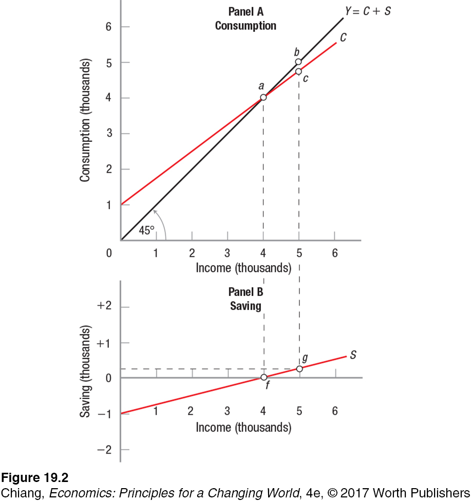
The saving schedule in panel B plots the difference between the 45° reference line (Y = C + S) and the consumption schedule in panel A. For example, if income is $4,000, saving is zero (point f in panel B), and when income equals $5,000, saving equals $250 [line (b − c) in panel A, point g in panel B]. Saving is positively sloped, again reflecting Keynes’s fundamental law; the more people earn, the greater percentage of income they will save (the average propensity to save rises as income rises). Make a mental note that the saving schedule shows how much people desire to save at various income levels.
How much people will actually save depends on equilibrium income, or how much income the economy is generating. We are getting a bit ahead of the story here, but planting this seed will help you when we get to the section where we determine equilibrium income in the economy.
Note finally that the consumption and saving schedules in our example are straight-
Other Determinants of Consumption and Saving Income is the principal determinant of consumption and saving, but other factors can shift the saving and consumption schedules. These factors include the wealth of a family, their expectations about the future of prices and income, family debt, and taxation.
Wealth The more wealth a family has, the higher its consumption at all levels of income. Wealth affects the consumption schedule by shifting it up or down, depending on whether wealth rises or falls. When the stock market was soaring in the late 1990s, policymakers worried about the wealth effect, that as many households saw their wealth dramatically expand, rising consumption might cause the economy’s inflation rate to rise. As it turned out, the stock market collapsed in 2000, and again in 2008, and the economy moved into recession. Then, economists began worrying about the negative impact of this wealth effect as trillions of dollars of wealth evaporated from the stock market before it eventually recovered.
Expectations Expectations about future prices and incomes help determine how much a person will spend today. If you anticipate that prices will rise next week, you will be more likely to purchase more products today. What are sales, after all, but temporary reductions in price designed to entice customers into the store today? Similarly, if you anticipate that your income will soon rise—
perhaps you are about to graduate from medical school— you will be more inclined to incur debt today to purchase something you want, as was the case with LeBron James, who drove an expensive Hummer while in high school, knowing that when he was drafted into the NBA, he would be making a fortune. Lotto winners who receive their winnings over a 20- year span often spend much of the money early on, running up debts. Few winners spend their winnings evenly over the 20 years. Household Debt Most households carry some debt, typically in the form of credit card balances, auto loans, student loans, or a home mortgage. The more debt a household has, the less able it is to spend in the current period as it makes payments toward the debt. Although the household might want to spend more money on goods now, its debt level restricts its ability to get more credit.
Taxes Taxes reduce disposable income, and therefore taxes result in reduced consumption and saving. When taxes are increased, spendable income falls; therefore, consumption is reduced by the MPC times the reduction in disposable income, and saving falls by the reduction in disposable income times the MPS. Tax reductions have the opposite effect, as we will see later in this chapter.
Investment
investment Spending by businesses that adds to the productive capacity of the economy. Investment depends on factors such as its rate of return, the level of technology, and business expectations about the economy.
When the town of West Point, Georgia, received the news that South Korean automaker Kia Motors was building a $1 billion car manufacturing facility in its town, its residents couldn’t have been happier. Not only was Kia creating thousands of jobs, the spending by its workers would create even more jobs throughout the region. Because Kia’s manufacturing facility was new to the U.S. economy (and not simply a move from another town), it is counted as gross private domestic investment (the “I” in the GDP equation), an important component of the aggregate expenditures model. Investment can come from foreign and domestic sources, for example, when American companies expand their operations by investing in new capital such as building a new factory.
Unlike consumer spending, which at 68% is the largest component of GDP and until recently held fairly steady from year to year, gross private domestic investment is volatile. Sure, large investment deals like Kia’s new plant in West Point, Georgia, are a huge boost to the economy, but such investments tend to be sporadic. The annual percentage changes in consumption and investment spending from 1980 to 2015 are shown in Figure 3.
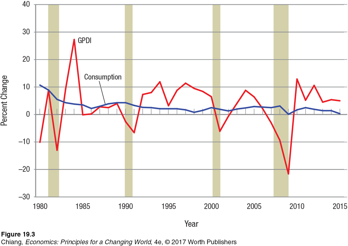

Notice that although consumption plodded along with annual increases between 0% and 10%, investment spending has undergone annual fluctuations ranging from −22% to +27%. Investment constitutes about 16% of GDP; therefore, its volatility often accounts for our recessions and booms.
The economic boom of the 1990s, for instance, was fueled by investments in information technology infrastructure, including massive investments in telecommunications. In the 1990s, people believed that Internet traffic would grow by 1,000% a year, doubling every three months or so. This belief led many companies to lay millions of miles of fiber optic cable. When the massive investments made in computer hardware and software over that same decade are taken into account, it is no wonder that the economy grew at a breakneck pace.
But this increase came to a halt in the early 2000s, when businesses—
Investment Demand Investment levels depend mainly on the rate of return on capital. Investments earning a high rate of return are the investments undertaken first (assuming comparable risk), with those projects offering lower returns finding their way into the investment stream later. Interest rate levels also are important in determining how much investment occurs, because much of business investment is financed through debt. As interest rates fall, investment rises, and vice versa.
Although the rate of return on investments is the main determinant of investment spending, other factors influence investment demand, including expectations, technological change, capital goods on hand, and operating costs.
Expectations Projecting the rate of return on investment is not an easy task. Returns are forecasted over the life of a new piece of equipment or factory, yet many changes in the economic environment can alter the actual return on these investments. As business expectations improve, investment demand will increase as businesses are willing to invest more at any given interest rate.
Technological Change Technological innovations periodically spur investment. The introduction of electrification, automobiles, and phone service at the beginning of the 20th century and, most recently, mobile technology and the new products they have spawned, are examples. Producing brand-
new products requires massive investments in plants, equipment, and research and development. These investments often take a long time before their full potential is realized. Operating Costs When the costs of operating and maintaining machinery and equipment rise, the rate of return on capital equipment declines and new investment will be postponed.
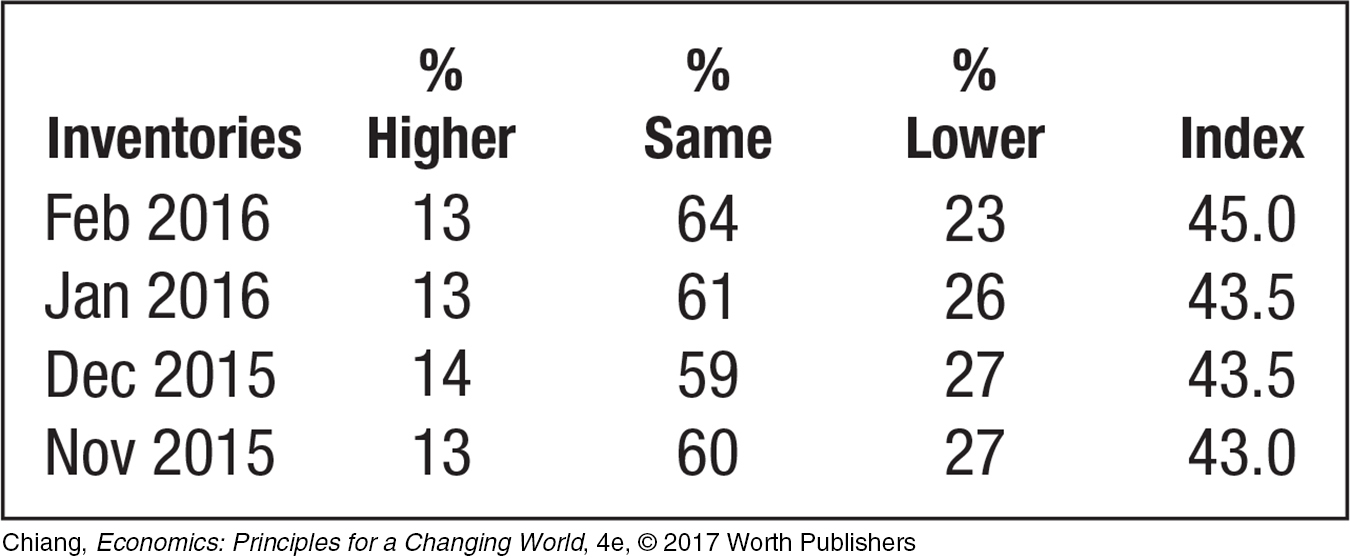
Capital Goods on Hand The more capital goods a firm has on hand, including inventories of the products it sells, the less the firm will want to make new investments. Until existing capacity can be fully used, investing in more equipment and facilities will do little to help profits.
Aggregate Investment Schedule To simplify our analysis, we will assume that rates of return and interest rates fully determine investment in the short run. But once that level of investment has been determined, it remains independent of income, or autonomous, as economists say. Therefore, unlike consumption, which increases as income rises, we will assume that investment does not vary based on income, but instead on the rates of return that determine how potentially profitable investment will be. Figure 4 shows the resulting aggregate investment schedule that plots investment spending with respect to income.
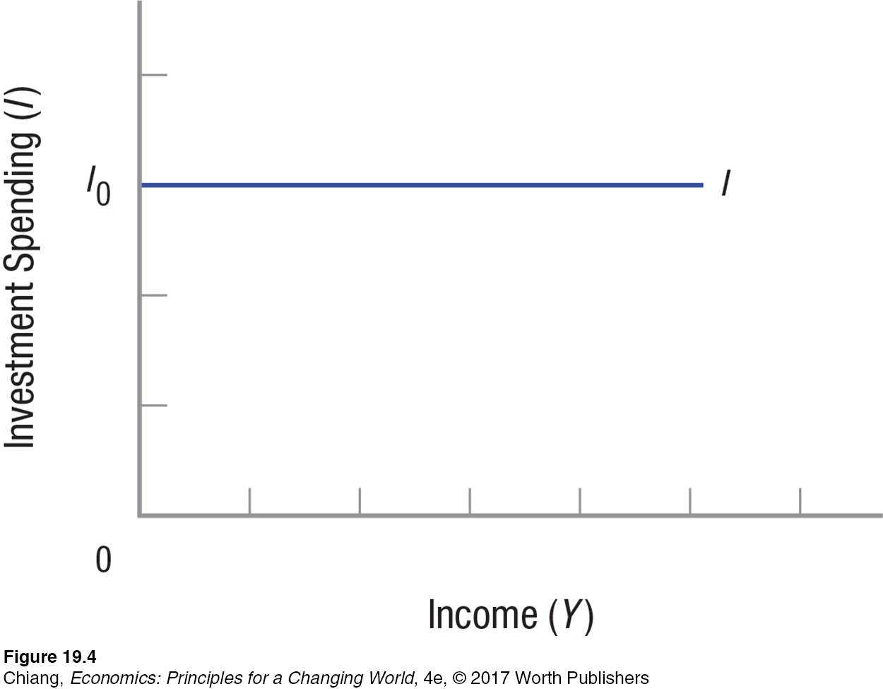
Because we have assumed that aggregate investment is I0 at all income levels, the curve is a horizontal straight line. Investment is unaffected by different levels of income. This is a simplifying assumption that we will change in later chapters when we look at its implications.
Our emphasis in this section has been on two important components of aggregate spending: consumption and investment. Consumption is about 68% and investment is about 16% of aggregate spending. Consumption is relatively stable, but investment is volatile and especially sensitive to expectations about conditions in the economy. We have seen that, on average, some income is spent (APC) and some is saved (APS). But, it is that portion of additional income that is spent (MPC) and saved (MPS) that is most important for where the economy settles or where it reaches equilibrium, as we will see in the next section.
CHECKPOINT
AGGREGATE EXPENDITURES
Aggregate expenditures are equal to C + I + G + (X − M), with consumption being about 68% of aggregate spending.
Keynes argued that saving and consumption spending are related to income. As income grows, consumption will grow but not as fast.
The marginal propensities to consume (MPC) and save (MPS) are equal to ΔC ÷ ΔY and ΔS ÷ ΔY, respectively. They represent the change in consumption and saving associated with a change in income.
Other factors affecting consumption and saving include wealth, expectations about future income and prices, the level of household debt, and taxes.
Investment levels depend primarily on the rate of return on capital.
Other determinants of investment demand include business expectations, technology change, operating costs, and the amount of capital goods on hand.
Consumption is relatively stable. In contrast, investment is volatile.
QUESTION: Why is investment spending generally much more volatile than consumption spending?
Answers to the Checkpoint questions can be found at the end of this chapter.
Consumer spending, while 5 times larger in absolute size than investment spending, involves many small expenditures by households that do not vary much from month to month, such as rent (or mortgage payment), food, and utilities. Consumers change habits, but slowly. Business investment expenditures are typically on big-