THE SIMPLE AGGREGATE EXPENDITURES MODEL
Now that we have stripped the government and foreign sectors from our analysis at this point, aggregate expenditures (AE) will consist of the sum of consumer and business investment spending (AE = C + I). Figure 5 shows a simple aggregate expenditures model based on consumption and investment. Aggregate expenditures based on the data in Table 1 are shown in panel A of Figure 5; panel B shows the corresponding saving and investment schedules.
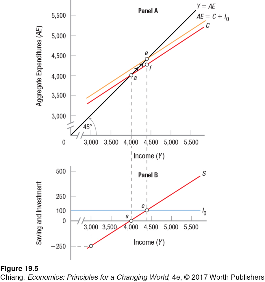
Let us take a moment to remind ourselves what these graphs represent. The 45° line in panel A represents the situation when income exactly equals spending, or Y = AE. In other words, no savings occur at any level of income. All other lines represent situations in which income does not exactly equal spending at all levels of income. Point a in both panels is that level of income ($4,000) at which saving is zero and all income is spent. Saving is therefore positive for income levels above $4,000 and negative at incomes below. The vertical distance ef in panel A represents investment (I0) of $100; it is equal to I0 in panel B. Note that the vertical axis of panel B has a different scale from that of panel A.
Macroeconomic Equilibrium in the Simple Model
Keynesian macroeconomic equilibrium The state of an economy at which all injections equal all withdrawals. There are no pressures pushing the economy to a higher or lower level of output.
The important question to ask is where this economy will come to rest. Or, in the language of economists, at what income will this economy reach Keynesian macroeconomic equilibrium? By equilibrium, economists mean that income at which there are no net pressures pushing the economy to move to a higher or lower level of output.
To find this equilibrium point, let’s begin with the economy at an income level of $4,000. Are there pressures driving the economy to grow or decline? Looking at point a in panel A of Figure 5, we see that the economy is producing $4,000 worth of goods and services and $4,000 in income. At this income level, however, consumers and businesses want to spend $4,100 ($4,000 in consumption and $100 in investment). Because aggregate expenditures (AE) exceed current income and output, there are more goods being demanded ($4,100) than are being supplied at $4,000. As a result, businesses will find it in their best interests to produce more, raising employment and income and moving the economy toward income and output level $4,400 (point e).
Once the economy has moved to $4,400, what consumers and businesses want to buy is exactly equal to the income and output being produced. Businesses are producing $4,400, aggregate expenditures are equal to $4,400, and there are no pressures on the economy to move away from point e. Income of $4,400, or point e, is an equilibrium point for the economy.
Panel B shows this same equilibrium, again as point e. Is it a coincidence that saving and investment are equal at this point where income and output are at equilibrium? The answer is no. In this simple private sector model, saving and investment will always be equal when the economy is in equilibrium.
JOHN MAYNARD KEYNES (1883–1946)
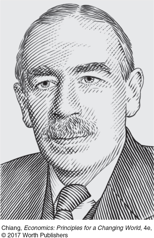
In 1935 John Maynard Keynes boasted in a letter to playwright George Bernard Shaw of a book he was writing that would revolutionize “the way the world thinks about economic problems.” This was a brash prediction to make, even to a friend, but it was not an idle boast. His General Theory of Employment, Interest and Money did change the way the world looked at economics.
Keynes belongs to a small class of economic earth-
Keynes was once asked if there was any era comparable to the Great Depression. He replied, “It was called the Dark Ages and it lasted 400 years.” His prescription to President Franklin D. Roosevelt was to increase government spending to stimulate the economy. Sundeep Reddy reports that “during a 1934 dinner . . . after one economist carefully removed a towel from a stack to dry his hands, Mr. Keynes swept the whole pile of towels on the floor and crumpled them up, explaining that his way of using towels did more to stimulate employment among restaurant workers” (The Wall Street Journal, January 8, 2009, p. A10).
During the world economic depression in the early 1930s, Keynes became alarmed when unemployment in England continued to rise after the first few years of the crisis. Keynes argued that aggregate expenditures, the sum of consumption, investment, government spending, and net exports, determined the levels of economic output and employment. When aggregate expenditures were high, the economy would foster business expansion, higher incomes, and high levels of employment. With low aggregate spending, businesses would be unable to sell their inventories and would cut back on investment and production.
The ideas formulated by Keynes dramatically changed the way government policy is used throughout the world. Today, as many countries face a slow economic recovery, governments have taken a more proactive role in their economies in hopes of avoiding another downturn of the magnitude seen in the 1930s.
Remember that aggregate expenditures are equal to consumption plus business investment (AE = C + I). Recall also that at equilibrium, aggregate expenditures, income, and output are all equal; what is demanded is supplied (AE = Y). Finally, keep in mind that income can either be spent or saved (Y = C + S). By substitution, we know that, at equilibrium,
AE = Y = C + I
We also know that
Y = C + S
Substituting C + I for Y yields
C + I = C + S
Canceling the C’s, we find that, at equilibrium,
I = S
Thus, the location of point e in panel B is not just coincidental; at equilibrium, actual saving and investment are always equal. Note that at point a, saving is zero, yet investment spending is $100 at I0. This difference means businesses desire to invest more than people desire to save. With desired investment exceeding desired saving, this cannot be an equilibrium point, because saving and investment must be equal in order for the economy to be at equilibrium. Indeed, income will rise until these two values are equal at point e.
What is important to take from this discussion? First, when intended (or desired) saving and investment differ, the economy will have to grow or shrink to achieve equilibrium. When desired saving exceeds desired investment—
injections Increments of spending, including investment, government spending, and exports.
withdrawals Activities that remove spending from the economy, including saving, taxes, and imports.
Second, at equilibrium all injections of spending (investment in this case) into the economy must equal all withdrawals (saving in this simple model). Spending injections increase aggregate income, while spending withdrawals reduce it. This fact will become important as we add government and the foreign sector to the model.
Returning to Figure 5, given an initial investment of $100 (I0), equilibrium is at an output of $4,400 (point e). Remember that at equilibrium, what people withdraw from the economy (saving) is equal to what others are willing to inject into the spending system (investment). In this case, both values equal $100. Point e is an equilibrium point because there are no pressures in the system to increase or decrease output; the spending desires of consumers and businesses are satisfied.
The Multiplier
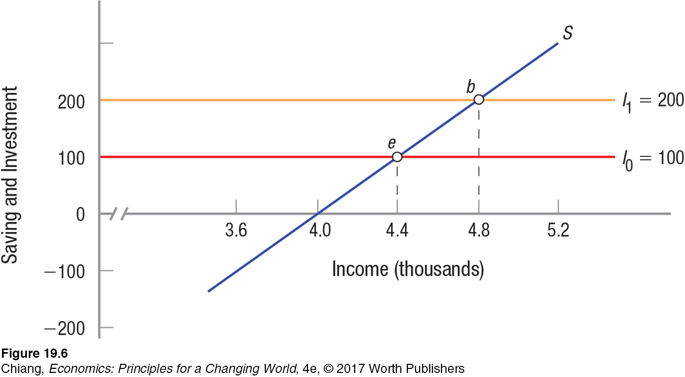
Injections and withdrawals in an economy produce an effect that is greater than the initial value of the injection or withdrawal. The following example illustrates why. Assume that full employment occurs at output $4,800. How much would investment have to increase to move the economy out to full employment? As Figure 6 shows, investment must rise to $200 (I1), an increase of $100. With this new investment, equilibrium output moves from point e to point b, and income rises from $4,400 to $4,800.
multiplier Spending changes alter equilibrium income by the spending change times the multiplier. One person’s spending becomes another’s income, and that second person spends some (the MPC), which becomes income for another person, and so on, until income has changed by 1/(1 − MPC) = 1/MPS. The multiplier operates in both directions.
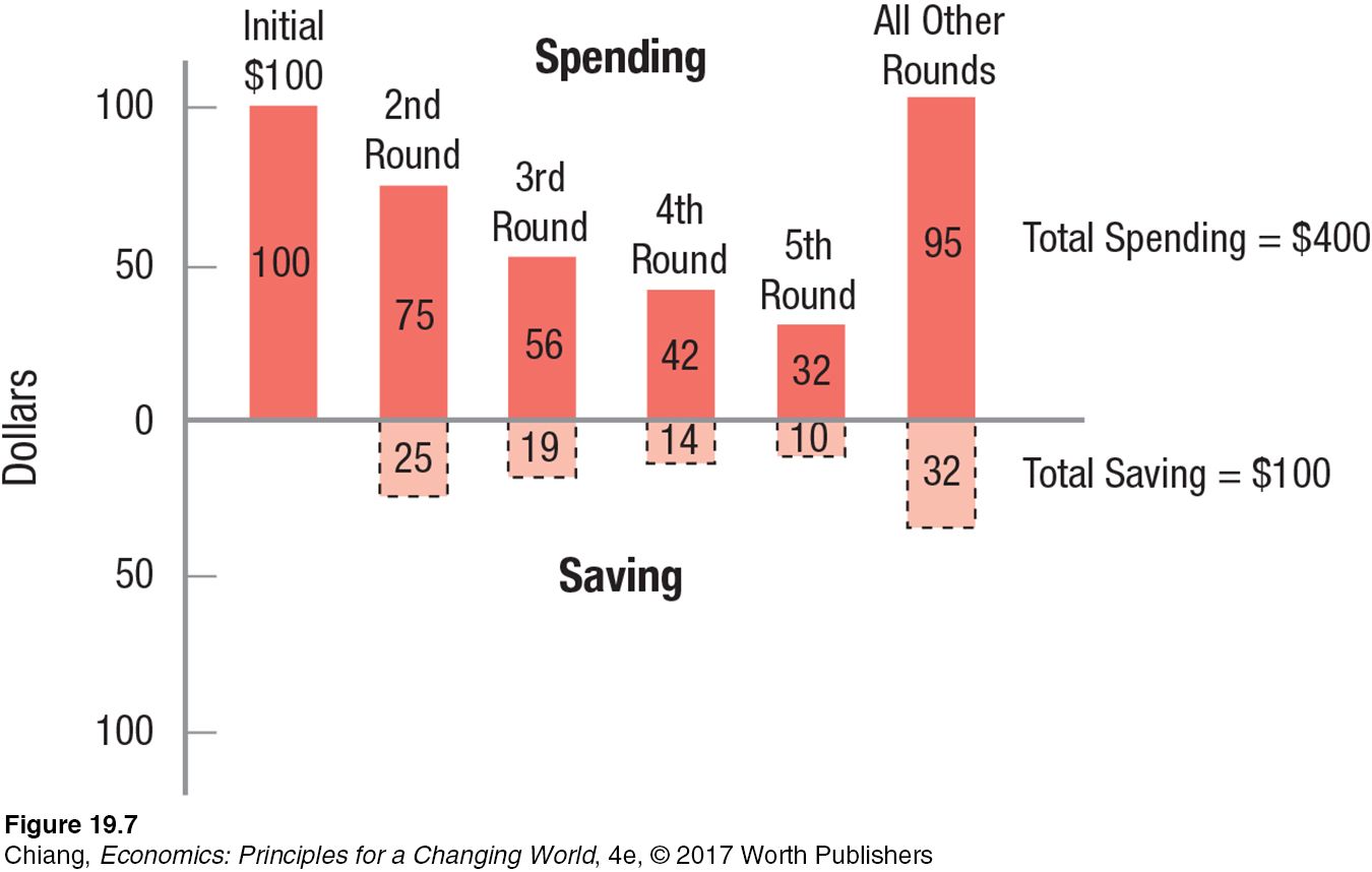
What is remarkable here is that a mere $100 of added spending (investment in this case) caused income to grow by $400. This phenomenon is known as the multiplier effect. Recognizing it was one of Keynes’s major insights. How does it work?
In this example, we have assumed the marginal propensity to consume is 0.75. Therefore, for each added dollar received by consumers, $0.75 is spent and $0.25 is saved. Thus, when businesses invest an additional $100, the firms providing the machinery will spend $75 of this new income on more raw materials, while saving the remaining $25. The firms supplying the new raw materials have $75 of new income. These firms will spend $56.25 of this (0.75 × $75.00), while saving $18.75 ($56.25 + $18.75 = $75.00). This effect continues on until the added spending has been exhausted. As a result, income will increase by $100 + $75 + $56.25 . . . . In the end, income rises by $400. Figure 7 outlines this multiplier process.
The general formula for the spending multiplier (k) is
k = 1/(1 – MPC)
Alternatively, because MPC + MPS = 1, the MPS = 1 − MPC; therefore,
k = 1/MPS
Thus, in our simple model, the multiplier is
1/(1 – 0.75) = 1/0.25 = 4
As a result of the multiplier effect, new spending will raise equilibrium by 4 times the amount of new spending. Note that any change in spending (consumption, investment—
The Multiplier Works in Both Directions
If spending increases raise equilibrium income by the increase times the multiplier, a spending decrease will reduce income in corresponding fashion. In our simple economy, for instance, a $100 decline in investment or consumer spending will reduce income by $400.
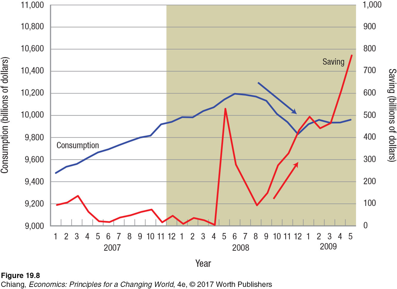
This is one reason why recession watchers are always concerned about consumer confidence. During a recession, income declines, or at least the rate of income growth falls. If consumers decide to increase their saving to guard against the possibility of job loss, they may inadvertently make the recession worse. As they pull more of their money out of the spending stream, withdrawals increase, and income is reduced by a multiplied amount as other agents in the economy feel the effects of this reduced spending. The result can be a more severe or longer-
This was the case when consumer spending peaked in the summer of 2008. After that, auto sales plummeted and housing prices and sales fell. As the recession that started in December 2007 progressed and jobs were lost, consumers reduced their spending. As their confidence in the economy deteriorated, households began to save more, consumer spending declined further, and the economy sank into a deeper recession. Figure 8 shows how consumer spending (downward arrow) fell and saving rose (upward arrow) after September 2008. Leading up to the recession, saving was less than 1% of personal income, but by mid-
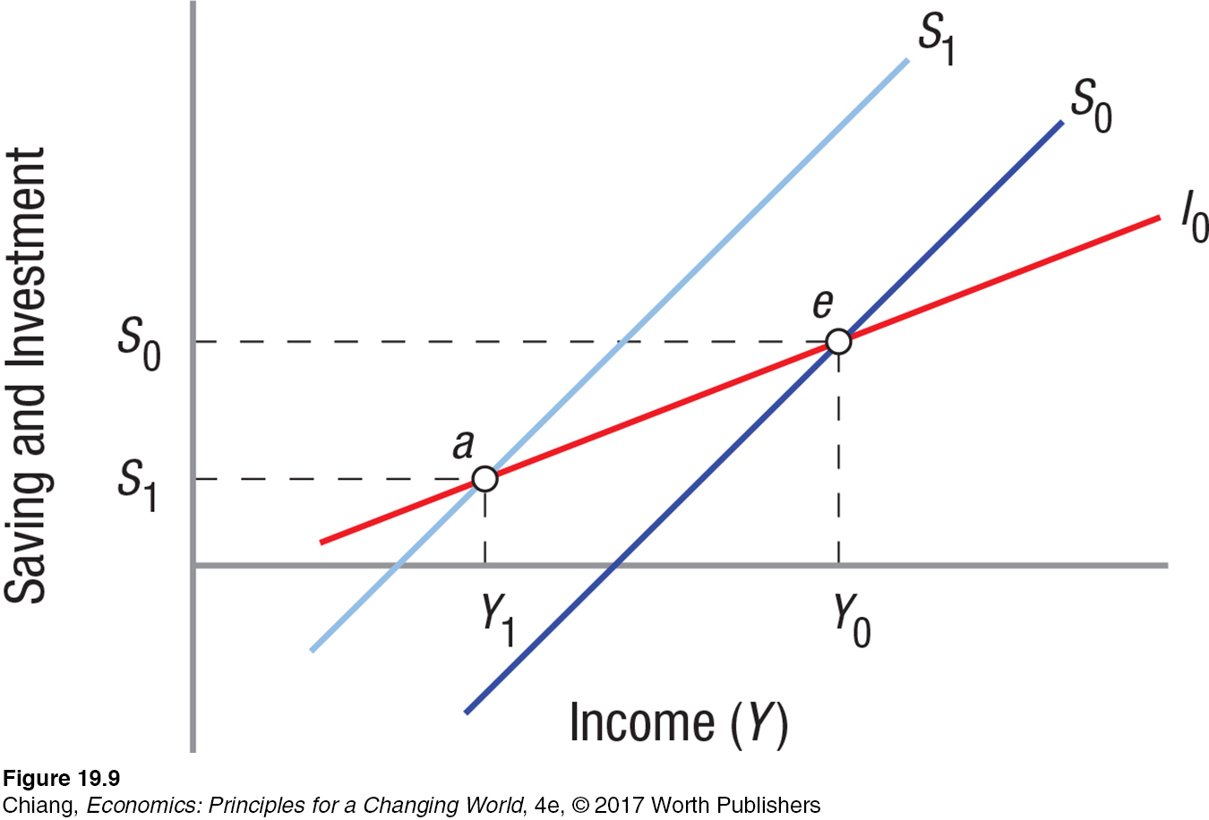
paradox of thrift When investment is positively related to income and households intend to save more, they reduce consumption. Consequently, income and output decrease, reducing investment such that savings actually end up decreasing.
Paradox of Thrift The implication of Keynesian analysis for actual aggregate household saving and household intentions regarding saving is called the paradox of thrift. As we saw in Figure 8, if households intend (or desire) to save more, they will reduce consumption, thereby reducing income and output, resulting in job losses and further reductions in income, consumption, business investment, and so on. The end result is an aggregate equilibrium with lower output, income, investment, and in the final analysis, lower actual aggregate saving.
Notice that we have modified our assumption about investment—
ISSUE
Do High Savings Rates Increase the Risk of a Long Recession?
Everyone has a frugal friend or relative who saves every penny possible, or a shopaholic friend who can’t seem to save any money at all. These differences in savings rates often are influenced by economic and demographic factors.

People with higher incomes tend to save a larger portion of their incomes than those with lower incomes. Older people tend to save more than younger people. And those living in rural areas tend to save more than those in urban areas. Yet, although these factors explain savings rates within a country, they do not fully explain the savings rate across countries. In other words, cultural differences play an important role as well.
The following bar graph shows the average household saving rate in a sample of twelve countries in 2016. China and India rank at the top of this list, despite having a lower income per capita than any other country on the list. The United States, which has the highest income per capita among the countries shown, has a savings rate toward the bottom. And some countries have seen dramatic changes in their savings rate, such as Japan, which had one of the highest savings rates 30 years ago, but today has the lowest savings rate among the countries shown.
The savings rate plays an important role in an economy. A high savings rate, such as that in China, India, and France, gives a country’s banking system a vote of confidence; people trust putting their money into financial institutions and expect the money will be available when desired. Also, savings provide opportunities for others to borrow, providing inexpensive access to loans for investment.
However, a high savings rate can also make a country vulnerable in times of recession. The adverse effects of a high savings rate are seen in China today, which has seen its growth rate fall in recent years. The natural reaction by Chinese citizens is to save even more, which may further slow economic growth and eventually lead to a recession. In the 1990s, Japan faced a decade-
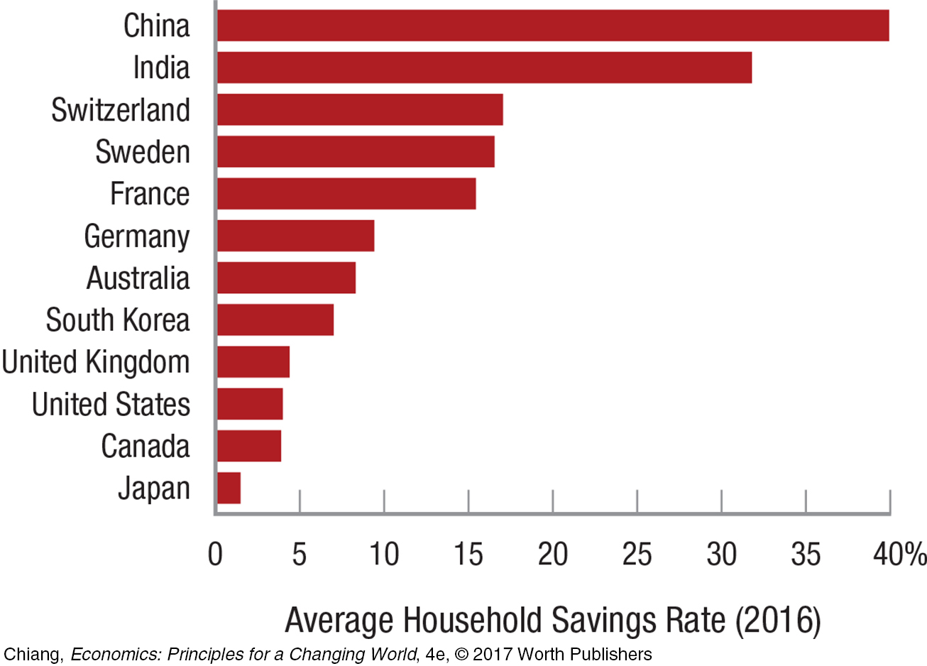
The ability of governments to minimize the effects of economic downturns depends on the marginal propensity to consume, which determines the multiplier. The higher the multiplier, the greater the effect government efforts to increase spending will have. Because China and India have very high savings rates, government incentives to boost consumption and investment may not be very effective, which doesn’t bode well should either country enter into a recession.
Initially, the economy is in equilibrium at point e with saving equal to S0. If households desire to save more because they feel insecure about their jobs, the savings curve will shift upward and to the left to S1. Now at all levels of income households intend to save more. This sets up the chain reaction described previously, leading to a new equilibrium at point a, where equilibrium income has fallen to Y1 and actual saving has declined to S1. The paradox is that if everyone tries to save more (even for good reasons), in the end they may end up saving less.

Brazil’s Beco Do Batman: How Graffiti Revived a Neighborhood
How did the Beco Do Batman neighborhood in São Paolo turn graffiti into an economic growth engine?
In cities around the world, graffiti artists exhibit their talents on the sides of buildings, trains, and bridges, turning otherwise pristine areas into unsightly views. Graffiti is also a common tool used by gangs, which increases the perception of neighborhoods with graffiti as unsafe, leading to a reduction in their desirability as a place to live or visit. As a result, neighborhoods and cities have an incentive to clean up graffiti. But because cleanup costs can be expensive and graffiti artists often return, winning the war against graffiti becomes difficult.
In one neighborhood in São Paulo, Brazil, instead of pumping more money into a never-

Instead of cleaning up the graffiti, residents encouraged graffiti artists to come to the area. Since the 1980s, artists from around Brazil and other countries journeyed to Beco Do Batman to paint giant murals in its alleyways. Because the lack of unpainted walls means that new artists must paint over a previous artist’s work, a constantly changing art gallery is created for visitors to enjoy. How did this strategy of welcoming graffiti affect the neighborhood?
First, overall crime declined. Because graffiti in Beco Do Batman was no longer a sign of gang power, criminal graffiti artists went elsewhere. This attracted wealthier residents and investors to build homes in the area, raising the property values of all homeowners and businesses.
Second, as Beco Do Batman became a unique tourist attraction, money was spent by tourists who visited the shops and restaurants in the area. The economic activity spurred by visitors created jobs and higher wages for its residents, who then had more money to spend. The cycle of increased economic activity generated a multiplier effect that allowed Beco Do Batman and its surrounding neighborhoods to thrive, pulling many of its residents out of poverty.
The graffiti art of Beco Do Batman is a unique example of how aggregate expenditures and the multiplier effect can lead to higher economic growth.
CHECKPOINT
THE SIMPLE AGGREGATE EXPENDITURES MODEL
Ignoring both the government and the foreign sector in a simple aggregate expenditures model, macroeconomic equilibrium occurs when aggregate expenditures are just equal to what is being produced.
At equilibrium, aggregate saving equals aggregate investment.
The multiplier process amplifies new spending because some of the new spending is saved and some becomes additional spending. And some of that spending is saved and some is spent, and so on.
The multiplier is equal to 1/(1 − MPC) = 1/MPS.
The multiplier works in both directions. Changes in spending are amplified, changing income by more than the initial change in spending.
The paradox of thrift results when households intend to save more, but at equilibrium they end up saving less.
QUESTION: Business journalists, pundits, economists, and policymakers all pay attention to the results of the Conference Board’s monthly survey of 5,000 households, called the Consumer Confidence Index. When the index is rising, this is good news for the economy, and when it is falling, concerns are often heard that it portends a recession. Why is this survey important as a tool in forecasting where the economy is headed in the near future?
Answers to the Checkpoint questions can be found at the end of this chapter.
When consumer confidence is declining, this may suggest that consumers are going to spend less and save more. Because consumer spending is about 68% of aggregate spending, a small decline represents a significant reduction in aggregate spending and may well mean that a recession is on the horizon. Relatively small changes in consumer spending coupled with the multiplier can mean relatively large changes in income, and therefore forecasters and policymakers should keep a close eye on consumer confidence.