THE FULL AGGREGATE EXPENDITURES MODEL
With the simple aggregate expenditures model of the domestic private sector (individual consumption and private business investment), we concluded that at equilibrium, saving would equal investment, and that changes in spending lead to a larger change in income. This multiplier effect was an important insight by Keynes. To build the full aggregate expenditures model, we now turn our attention to adding government spending and taxes and the impact of the foreign sector.
Adding Government Spending and Taxes
Although government spending and tax policy can get complex, for our purposes it involves simple changes in government spending (G) or taxes (T ). As we have seen in the previous section, any change in aggregate spending causes income and output to rise or fall by the spending change times the multiplier.
Figure 10 illustrates a change in government spending. Initially, investment is $100; therefore, equilibrium income is $4,400 (point e), just as in Figure 6 earlier. Rather than investment rising by $100, let’s assume that the government decides to spend another $100. As Figure 10 shows, the new equilibrium is $4,800 (point b). This result is similar to the one in Figure 6, confirming that spending is spending; the economy does not care where it comes from.
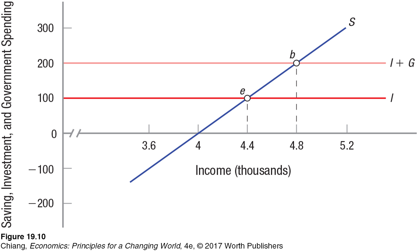
A quick summary is now in order. Equilibrium income is reached when injections (here, I + G = $200) equal withdrawals (in this case, S = $200). It did not matter whether these injections came from investment alone or from investment and government spending together. The key is spending.
Changes in spending modify income by an amount equal to the change in spending times the multiplier. How, then, do changes in taxes affect the economy? The answers are not as simple in that case.
Tax Changes and Equilibrium When taxes are increased, money is withdrawn from the economy’s spending stream. When taxes are reduced, money is injected into the economy’s spending stream because consumers and businesses have more to spend. Thus, taxes form a wedge between income and that part of income that can be spent, or disposable income. Disposable income (Yd) is equal to income minus taxes (Yd = Y − T ). For simplicity, we will assume that all taxes are paid in a lump sum, thereby removing a certain fixed sum of money from the economy. This assumption does away with the need to worry now about the incentive effects of higher or lower tax rates.
Returning to the model of the economy we have been developing, consumer spending now relates to disposable income (Y − T ), rather than just income. Table 2 reflects this change, using disposable income to determine consumption. With government spending and taxes (fiscal policy) in the model, spending injections into the economy include government spending plus business investment (G + I ). Withdrawals from the system include saving and taxes (S + T ).
| TABLE 2 | KEYNESIAN EQUILIBRIUM ANALYSIS WITH TAXES | |||||
| Income or Output (Y ), in $ | Taxes (T ), in $ | Disposable Income (Yd ), in $ | Consumption (C ) | Saving (S ) | Investment (I ) | Government Spending (G ) |
| 4,000 | 100 | 3,900 | 3,925 | −25 | 100 | 100 |
| 4,100 | 100 | 4,000 | 4,000 | 0 | 100 | 100 |
| 4,200 | 100 | 4,100 | 4,075 | 25 | 100 | 100 |
| 4,300 | 100 | 4,200 | 4,150 | 50 | 100 | 100 |
| 4,400 | 100 | 4,300 | 4,225 | 75 | 100 | 100 |
| 4,500 | 100 | 4,400 | 4,300 | 100 | 100 | 100 |
| 4,600 | 100 | 4,500 | 4,375 | 125 | 100 | 100 |
| 4,700 | 100 | 4,600 | 4,450 | 150 | 100 | 100 |
| 4,800 | 100 | 4,700 | 4,525 | 175 | 100 | 100 |
| 4,900 | 100 | 4,800 | 4,600 | 200 | 100 | 100 |
| 5,000 | 100 | 4,900 | 4,675 | 225 | 100 | 100 |
Again, equilibrium requires that injections equal withdrawals, or in this case,
G + I = S + T
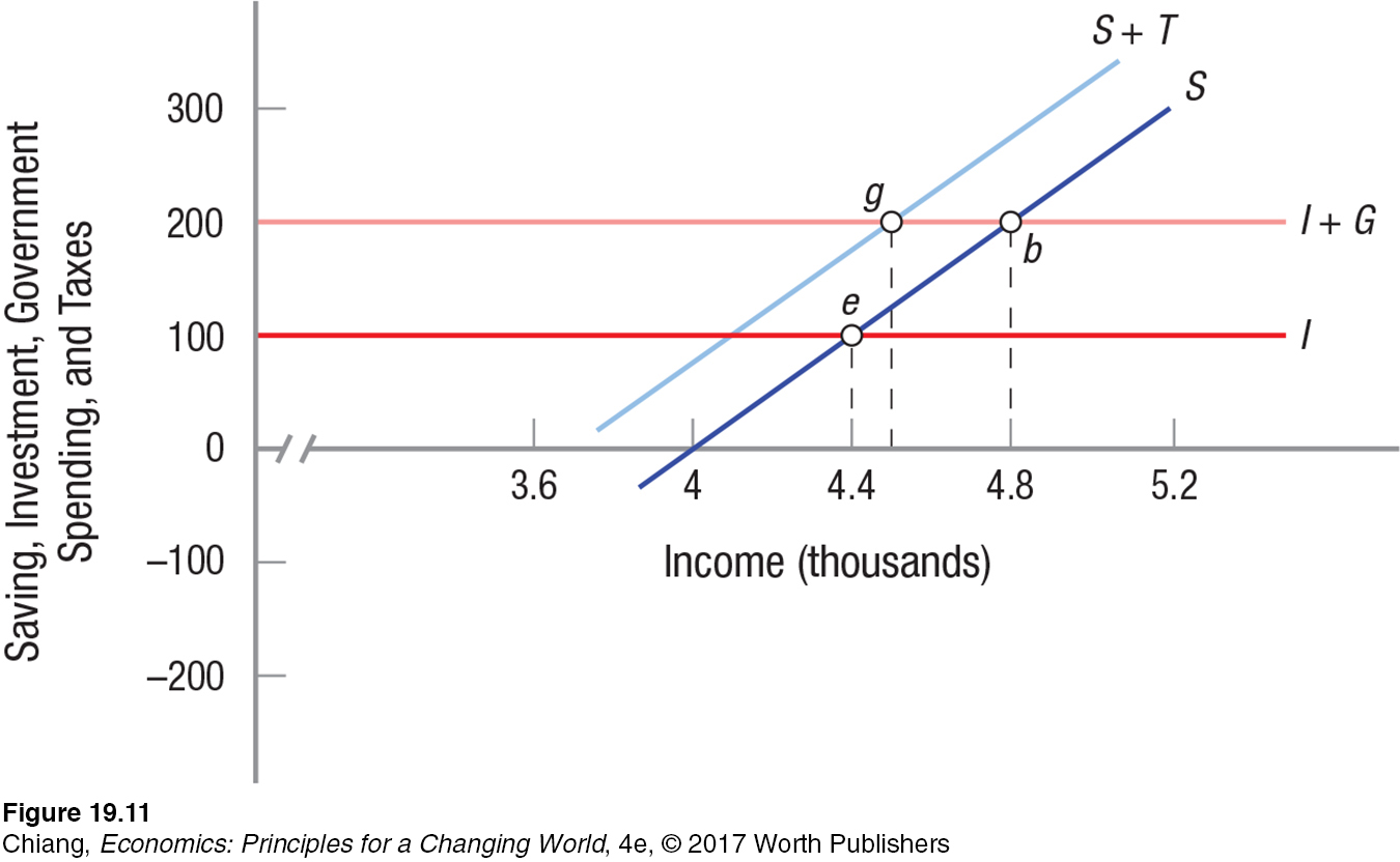
In our example, Table 2 shows that G + I = S + T at income level $4,500 (the shaded row in the table). If no tax had been imposed, equilibrium would have been at the point at which S = G + I, and thus at an income of $4,800 (point b in Figure 10, not shown in Table 2). Therefore, imposing the tax reduces equilibrium income by $300. Because taxes represent a withdrawal of spending from the economy, we would expect equilibrium income to fall when a tax is imposed. Yet, why does equilibrium income fall by only $300, and not by the tax multiplied by the multiplier, which would be $400?
The answer is that consumers pay for this tax, in part, by reducing their saving. Specifically, with the MPC at 0.75, the $100 tax payment is split between consumption, reduced by $75, and saving, reduced by $25. When this $75 decrease in consumption is multiplied by the multiplier, this yields a decline in income of $300 ($75 × 4). The reduction in saving of $25 dampens the impact of the tax on equilibrium income because those funds were previously withdrawn from the spending stream. Changing the withdrawal category from saving to taxes does not affect income: Both are withdrawals.
Equilibrium is shown at point g in Figure 11. At point g, I + G = S + T, with equilibrium income equal to $4,500 and taxes and saving equal to $100 each.
The result is that a tax increase (or decrease, for that matter) will have less of a direct impact on income, employment, and output than will an equivalent change in government spending. For this reason, economists typically describe the “tax” multiplier (calculated as MPC/(1 − MPC)) as being smaller than the “spending” multiplier (1/(1 − MPC)).
The Balanced Budget Multiplier By now you have probably noticed a curious thing. Our original equilibrium income was $4,400, with investment and saving equal at $100. When the government was introduced with a balanced budget (G = T = $100), income rose by $100 to $4,500, while equilibrium saving and investment remained constant at $100.
balanced budget multiplier Equal changes in government spending and taxation (a balanced budget) lead to an equal change in income (the balanced budget multiplier is equal to 1).
This has led to what economists call the balanced budget multiplier. Equal changes in government spending and taxation (a balanced budget) lead to an equal change in income. Equivalently, the balanced budget multiplier is equal to 1. If spending and taxes are increased by the same amount, income grows by this amount, hence a balanced budget multiplier equal to 1. Note that the balanced budget multiplier is 1 no matter what the values of MPC and MPS.
Adding Net Exports
Thus far we have essentially assumed a closed economy by avoiding adding foreign transactions: exports and imports. We now add the foreign sector to complete the aggregate expenditures model.
The impact of the foreign sector in the aggregate expenditures model is through net exports: exports minus imports (X − M ). Exports are injections of spending into the domestic economy, and imports are withdrawals. When Africans purchase grain from American farmers, they are injecting new spending on grain into our economy. Conversely, when we purchase French wine, we are withdrawing spending (as saving does) and injecting these funds into the French economy.
Figure 12 adds net exports to Figure 10 with investment and government spending. By adding $100 of net exports to the previous equilibrium at point b, equilibrium moves to $5,200 (point c). Again, we see the multiplier at work as the $100 in net exports leads to a $400 increase in income.
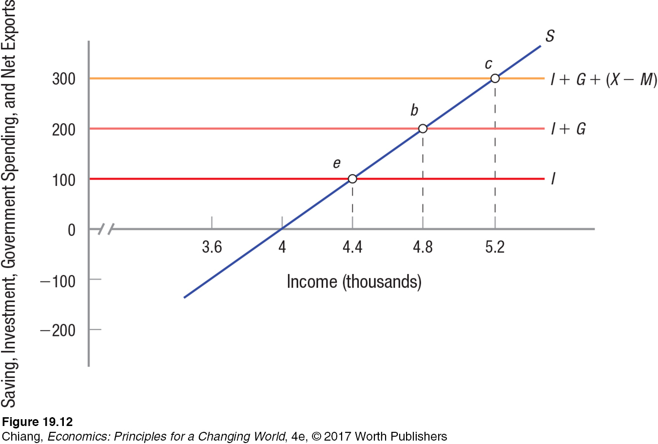
With the foreign sector included, all injections into the economy must equal all withdrawals; therefore at equilibrium,
I + G + X = S + T + M
Thus, if we import more and all other spending remains the same, equilibrium income will fall. This is one reason why many economists focus on the trade deficit or net exports (X − M ) figures each month.
The aggregate expenditures model illustrates the importance of spending in an economy. Investment, government spending, and exports all increase income, whereas saving, taxes, and imports reduce it. Further, the fact that consumers spend and save some of the changes in income (MPC and MPS) gives rise to a spending multiplier that magnifies the impact of changes in spending on the economy.
Recessionary and Inflationary Gaps
Keynesian analysis illustrated what was needed to get the economy out of the Great Depression: an increase in aggregate spending. Without an increase in spending, an economy can be stuck at a point below full employment for an extended period of time. Therefore, Keynes argued that if consumers, businesses, and foreigners were unwilling to spend (their economic expectations were clearly dismal), government should. This was also the basic rationale for the extraordinary spending measures implemented by Congress and signed by President Obama during the 2007–
recessionary gap The increase in aggregate spending needed (when expanded by the multiplier) to bring a depressed economy back to full employment.
Recessionary Gap The recessionary gap is the increase in aggregate spending needed to bring a depressed economy back to full employment. Note that it is not the difference between real GDP at full employment and current real GDP, which is called the GDP gap. If full employment income is $4,400 and our current equilibrium income is $4,000, the recessionary gap is the added spending ($100) that when boosted by the multiplier (4 in this case) will close a GDP gap ($400).
inflationary gap The spending reduction necessary (when expanded by the multiplier) to bring an overheated economy back to full employment.
Inflationary Gap If aggregate spending generates income above full employment levels, the economy will eventually heat up, creating inflationary pressures. Essentially, the economy is trying to produce more output and income than it can sustain for very long. Thus, the excess aggregate spending exceeding that necessary to result in full employment is the inflationary gap. Using our previous example, if full employment is an income of $4,400 and our current equilibrium is $4,800, a reduction in spending is needed to close the $400 GDP gap and to prevent inflation from building. In this case, a reduction in aggregate expenditures of $100 with a multiplier of 4 would bring the economy back to full employment at $4,400. In sum, changes in aggregate expenditures expanded by the multiplier can help bring an economy facing either recessionary or inflationary pressures back into equilibrium sooner.
This Keynesian approach to analyzing aggregate spending revolutionized the way economists looked at the economy and led to the development of modern macroeconomics. In the next chapter, we extend our analysis to the aggregate demand and supply model, a modern extension of this aggregate expenditures model to account for varying price levels and the supply side of the macroeconomy.
ISSUE
Was Keynes Right About the Great Depression?
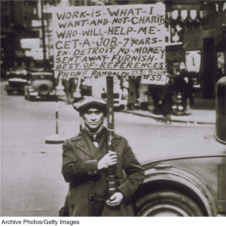
There is little disagreement that the Great Depression was one of the most important events in the United States in modern history. Good aggregate data were not yet available, but President Roosevelt and congressional leaders knew something was very wrong.
Within a couple of years, 10,000 banks collapsed, farms and businesses were lost, the stock market lost 85% of its value from the beginning of the decade, and soup kitchens fed a growing horde as unemployment soared to nearly 25%, up from 3.2% in 1929. Worse, the Great Depression persisted: It did not look to be temporary; there was no end in sight.
The aggregate expenditures model we have just studied provides some insight into the Great Depression. The figure plots hypothetical saving and investment curves over the actual data for 1929 and 1933. Both government and the foreign sector were tiny at this time; therefore, the simple aggregate expenditures model effectively illustrates why the Great Depression did not show signs of much improvement; by 1939 the unemployment rate was still over 17%.
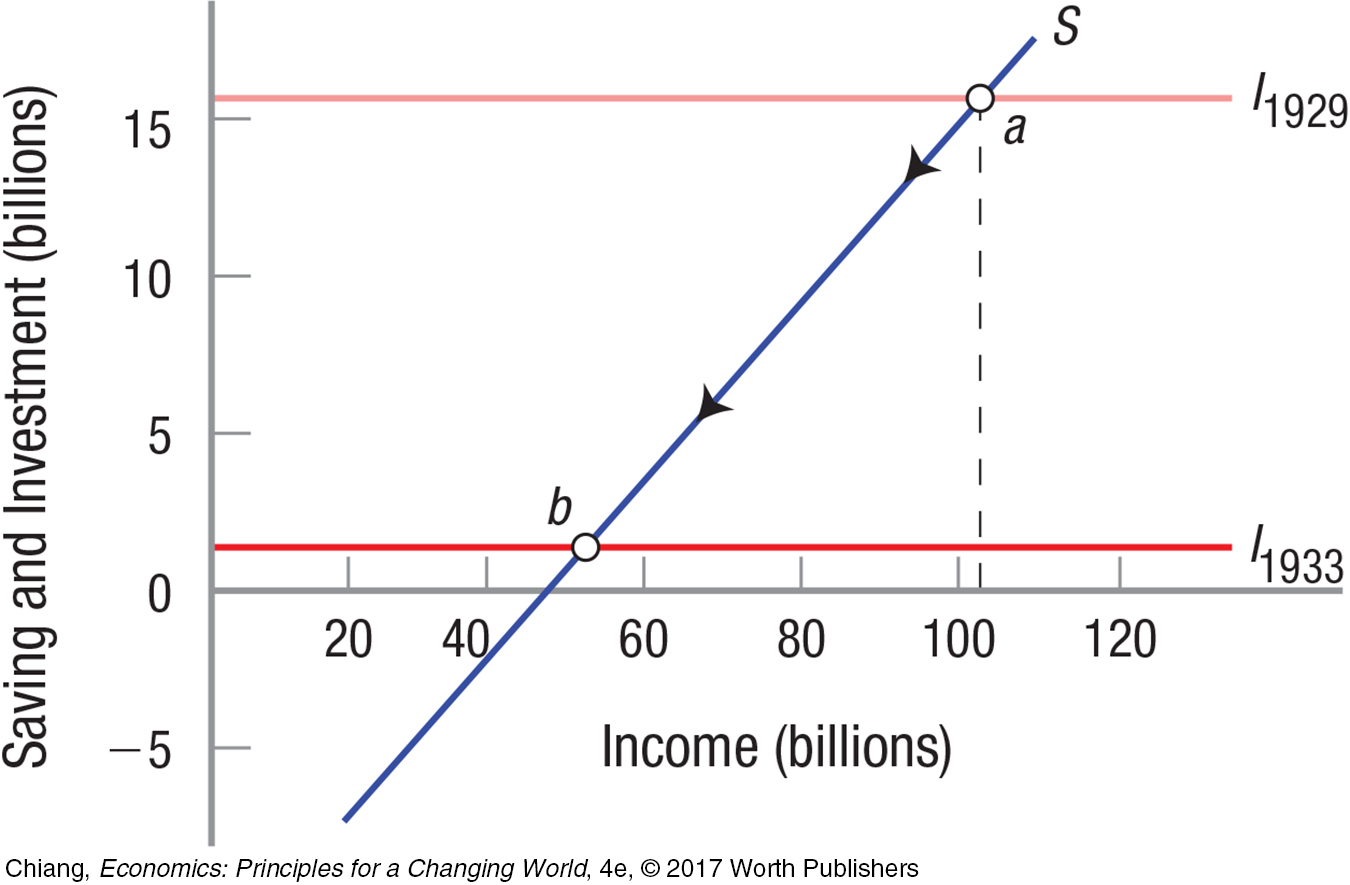
Saving and investment were over $16 billion in 1929, or roughly a healthy 15% of GDP (point a). By 1933 investment collapsed to just over $1 billion (a 91% decline), and the economy was in equilibrium at an income of roughly half of that in 1929 (point b). Government spending remained at roughly the same levels while net exports, a small fraction of aggregate expenditures, fell by more than half of their previous levels.
Keynes had it right: Unless something happened to increase investment or exports (not likely given that the rest of the world was suffering economically as well), the economy would remain mired in the Great Depression (point b). He suggested that government spending was needed. Ten years later (1943), the United States was in the middle of World War II, and aggregate expenditures swelled as government spending rose by a factor of 10. The Great Depression was history.
CHECKPOINT
THE FULL AGGREGATE EXPENDITURES MODEL
Government spending affects the economy in the same way as other spending.
Tax increases withdraw money from the spending stream but do not affect the economy as much as spending reductions, because these tax increases are partly offset by decreases in saving.
Tax decreases inject money into the economy but do not affect the economy as much as spending increases, because tax reductions are partly offset by increases in saving.
Equal changes in government spending and taxes (a balanced budget) result in an equal change in income (a balanced budget multiplier of 1).
A recessionary gap is the new spending required that, when expanded by the multiplier, moves the economy to full employment.
An inflationary gap is the spending reduction necessary (again when expanded by the multiplier) to bring the economy back to full employment.
QUESTIONS: If the government is considering reducing taxes to stimulate the economy, does it matter if the MPS is 0.25 or 0.33? What if the government reduces government spending by an equal amount to fund the tax cut?
Answers to the Checkpoint questions can be found at the end of this chapter.
Yes, it does matter. If the tax reduction is going to be $100, for example, and the MPS is 0.25, the multiplier is 4, and the income increase will be $75 × 4 = $300. Keep in mind that in this case, one-