AGGREGATE SUPPLY

537

aggregate supply The real GDP that firms will produce at varying price levels. The aggregate supply curve is positively sloped in the short run but vertical in the long run.

The aggregate supply curve shows the real GDP that firms will produce at varying price levels. Even though the definition seems similar to that for aggregate demand, note that we have now moved from the spending side of the economy to the production side. We will consider two different possibilities for aggregate supply: the short run and the long run. In the short run, aggregate supply is positively sloped and prices rise when GDP grows. In contrast, long-run aggregate supply reflects the long-run state of the economy and is represented by a vertical curve. Growth occurs in the economy by shifting this vertical aggregate supply curve to the right. Let’s begin by looking at the economy from the long-run perspective.

Long Run

long-run aggregate supply (LRAS) curve The long-run aggregate supply curve is vertical at full employment because the economy has reached its capacity to produce.

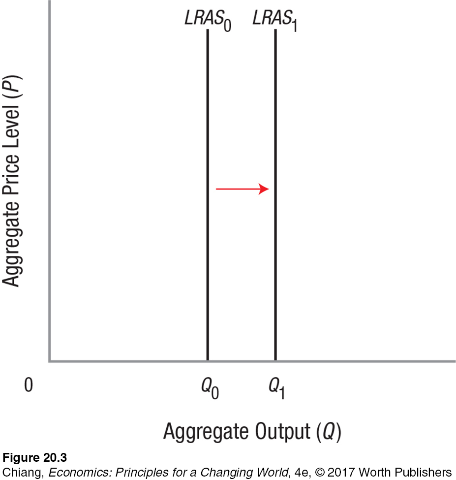
The vertical long-run aggregate supply (LRAS) curve incorporates the assumptions of classical (pre-1930s) economic analysis. Classical analysis assumes that all variables are adjustable in the long run, where product prices, wages, and interest rates are flexible. As a result, the economy will gravitate to the position of full employment shown as Q0 in Figure 3.

Figure 20.3: FIGURE 3 LONG-RUN AGGREGATE SUPPLY
image
Figure 20.3: The long-run aggregate supply (LRAS) curve is vertical, reflecting the assumptions of classical economic analysis. In the long run, all variables in the economy can adjust, and the economy will settle at full employment at output Q0. Changes in the amount of resources available, the quality of the labor force, and technology can shift the LRAS curve to the right to LRAS1, at a new full employment output at Q1.

Full employment is often referred to as the natural rate of output or the natural rate of unemployment by economists. This long-run output is an equilibrium level at which inflationary pressures are minimal. Once the economy has reached this level, further increases in output are extremely difficult to achieve; there is no one else to operate more machines, and no more machines to operate. As we will see later, attempts to expand beyond this output level only lead to higher prices and rising inflation.

In general terms, the vertical LRAS curve represents the full employment capacity of the economy and depends on the amount of resources available for production and the available technology. Full employment is determined by the capital available, the size and quality of the labor force, and the technology employed; in effect, the productive capacity of the economy. Remember from earlier chapters that these are also the big three factors driving economic growth (shifting the LRAS0 curve to the right to LRAS1) once a suitable infrastructure has been put in place.

Determinants of Long-Run Aggregate Supply

538

Attempts to improve technology such as automation and digitalization are clear examples of an increase in productive capacity. But so is the enhancement of labor quality. As a greater percentage of people pursue college and postgraduate degrees, productivity increases and leads to economic growth. Finally, increased trade and globalization have allowed resources to flow more freely, permitting the United States to gain access to better or cheaper inputs and more specialized labor.

Each of the shifts in the LRAS curve takes time. It’s not easy to improve the human capital of an entire nation or to develop new production technologies. Therefore, although the LRAS is of concern to the long-term welfare of the country, policymakers are often more concerned about short-run outcomes. We now turn to the short-run aggregate supply (SRAS) curve.

Short Run

short-run aggregate supply (SRAS) curve The short-run aggregate supply curve is positively sloped because many input costs are slow to change (sticky) in the short run.

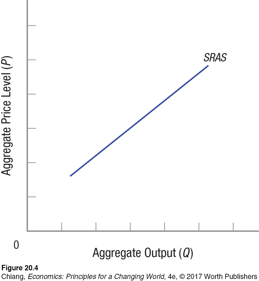
Figure 4 shows the short-run aggregate supply (SRAS) curve, which is positively sloped because some input costs are slow to change in the short run. When prices rise, firms do not immediately see an increase in wages or rents because these are often fixed for a specified term; in other words, input prices are sticky. Thus, profits will rise with the rising prices and firms will supply more output as their profits increase.

Figure 20.4: FIGURE 4 SHORT-RUN AGGREGATE SUPPLY
image
Figure 20.4: The short-run aggregate supply (SRAS) curve is positively sloped because many input costs are slow to change in the short run (they are sticky).

This situation, however, cannot last for long. As an entire industry or the economy as a whole increases its production, firms must start hiring more labor or paying overtime. As each firm seeks more employees, wages are driven up, increasing costs and forcing higher prices.

For the economy as a whole, a rise in real GDP results in higher employment and reduced unemployment. Lower unemployment rates mean a tightening of labor markets. This often leads to fierce collective bargaining by labor, followed by increases in wages, costs, and prices. The result is that a short-run increase in GDP is usually accompanied by a rise in the price level.

Determinants of Short-Run Aggregate Supply

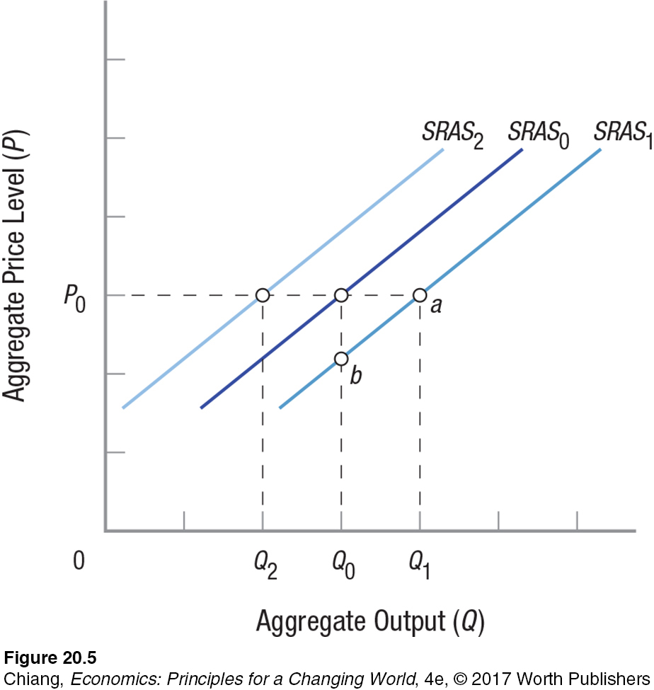
We have seen that, because the aggregate supply curve is positively sloped in the short run, a change in aggregate output, other things held constant, will result in a change in the aggregate price level. The determinants of short-run aggregate supply—those other things held constant—include changes in input prices, productivity, taxes, regulation, the market power of firms, or business and inflationary expectations. When any of these determinants change, the entire SRAS curve shifts, as Figure 5 illustrates.

Figure 20.5: FIGURE 5 SHIFTS IN SHORT-RUN AGGREGATE SUPPLY
image
Figure 20.5: The determinants of short-run aggregate supply include changes in input prices, productivity, taxes, regulation, the market power of firms, and inflationary expectations. If one of these determinants changes, the entire short-run aggregate supply curve shifts. Increasing productivity, for instance, will shift the short-run aggregate supply curve to the right, from SRAS0 to SRAS1. Conversely, raising taxes or adding inefficient regulations can shift the short-run aggregate supply curve to the left, from SRAS0 to SRAS2.

539

image
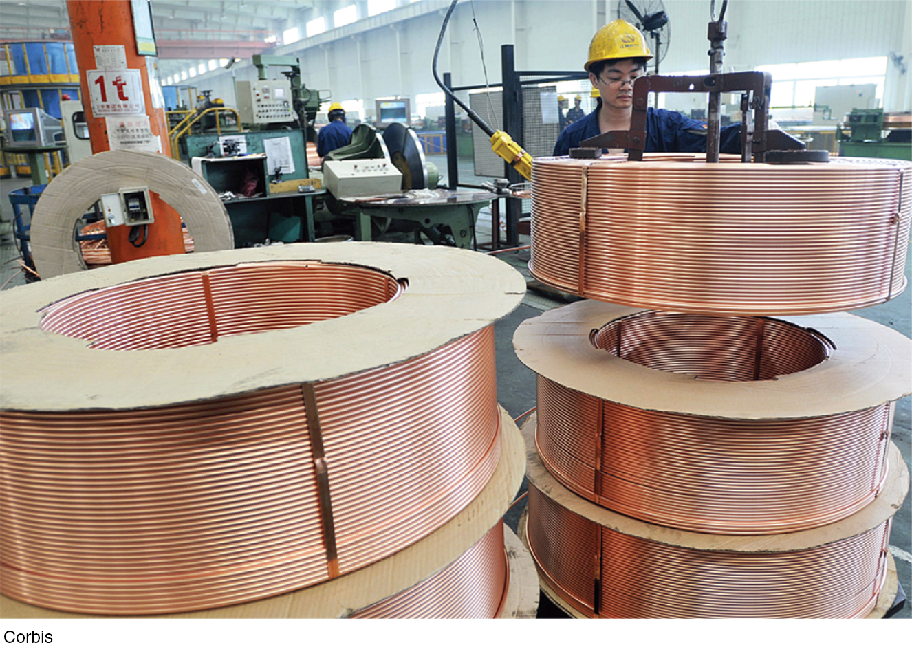
The dramatic rise in copper prices from 2006 to 2012 increased the cost of producing copper products, and contributed to a decrease in aggregate supply.
Corbis

Input Prices Changes in the cost of land, labor, or capital will change the output that firms are willing to provide to the market. When world crude oil prices rise, it is never long before prices rise at the gasoline pump. Rising input prices are quickly passed along to consumers, and the opposite is true as well. New discoveries of raw materials result in falling input prices, causing the prices for products incorporating these inputs to drop. This means that more of these products can be produced at a price of P0 in Figure 5 as short-run aggregate supply shifts to SRAS1 (point a), or now output Q0 can be produced at a lower price on SRAS1 (point b).

Productivity Changes in productivity are another major determinant of short-run aggregate supply. Rising productivity will shift the short-run aggregate supply curve to the right—from SRAS0 to SRAS1 in Figure 5—and vice versa. This is why changes in technology that increase productivity are so important to the economy. Technological advances, moreover, often lead to new products that expand short-run aggregate supply. The willingness of firms to invest in new capital equipment (aided by an improved business outlook) will enhance the productive capacity of an economy, which can also increase long-run aggregate supply.

An example of a technological advance is the improvement in traffic-enhanced GPS navigational devices, which allows one to select the quickest route to a destination taking into account traffic and roadblocks (such as those caused by construction projects and car crashes) in real time. Such technological enhancements let commercial vehicles reduce their time on the road, reducing transportation costs to the company. These cost reductions lead to an increase in short-run aggregate supply. If these technologies expand the overall productive capacity of the economy, they can also increase long-run aggregate supply.

540

Taxes and Regulation Rising taxes or increased regulation can shift the short-run aggregate supply curve to the left, from SRAS0 to SRAS2 in Figure 5. Excessively burdensome regulation, though it may provide some benefits, raises costs so much that the new costs exceed the benefits. This results in a decrease in short-run aggregate supply. Often, no one knows how much regulation has increased costs until some sort of deregulation is instituted.

Alternatively, tax reductions such as investment tax credits reduce the costs of production, resulting in an increase in short-run aggregate supply. Similarly, improving the process of satisfying regulations, such as reducing required paperwork, also can increase short-run aggregate supply even when the regulations themselves do not change.

Market Power of Firms Monopoly firms charge more than competitive firms. Therefore, a change in the market power of firms can increase prices for specific products, thereby reducing short-run aggregate supply. When the Organization of Petroleum Exporting Countries (OPEC) formed in 1973, it raised oil prices by over 200% within three years by reducing the global supply of oil. Because at that time there were very few substitutes for oil, higher oil prices shifted the SRAS curve to the left.

Today, with many non-OPEC nations (such as Russia, Norway, and Canada) producing large quantities of oil, OPEC’s power to raise prices has fallen.

Inflationary Expectations A change in inflationary expectations by businesses, workers, or consumers can shift the short-run aggregate supply curve. If, for example, workers believe that inflation is going to increase, they will bargain for higher wages to offset the expected losses to real wages. The intensified bargaining and resulting higher wages will reduce aggregate supply.

To summarize, the short-run aggregate supply curve slopes upward because many input costs are slow to change (i.e., are sticky) in the short run. This SRAS curve can shift because of changes in input prices, productivity, taxes, regulation, the market power of firms, or inflationary expectations. Table 2 summarizes the determinants of short-run aggregate supply.

TABLE 2 DETERMINANTS OF SHORT-RUN AGGREGATE SUPPLY (THE SHORT-RUN AGGREGATE SUPPLY CURVE SHIFTS WHEN THESE CHANGE)
Determinant SRAS Increases SRAS Decreases
Changes in Input Prices Prices decline Prices rise
Changes in Productivity
  • Technology

Improvements Reductions
  • Changes in human capital

Improvements Reductions
Changes in Taxes and Regulations
  • Tax rates

Lower Higher
  • Subsidies

Higher Lower
  • Change in burdensome regulations

Reductions Additions
Change in Market Power Reductions Increases
Changes in Inflationary Expectations Lower Higher
Table 20.2: TABLE 2 DETERMINANTS OF SHORT-RUN AGGREGATE SUPPLY (THE SHORT-RUN AGGREGATE SUPPLY CURVE SHIFTS WHEN THESE CHANGE)

541

CHECKPOINT

AGGREGATE SUPPLY

  • The aggregate supply curve shows the real GDP that firms will produce at varying price levels.

  • The vertical long-run aggregate supply (LRAS) curve represents the long-run full-employment capacity of the economy.

  • Increasing resources or improved technology shift the LRAS curve, which represents economic growth.

  • The short-run aggregate supply (SRAS) curve is upward-sloping, reflecting rigidities in the economy because input and output prices are slow to change (sticky).

  • The determinants of short-run aggregate supply include changes in input prices, productivity, taxes, regulations, the market power of firms, and inflationary expectations.

QUESTION: Because interest rates had been kept extremely low for almost a decade, many investors worried that access to cheap loans will drive prices higher as more people borrow money for purchases. How might this change in inflationary expectations affect the SRAS curve?

Answers to the Checkpoint questions can be found at the end of this chapter.

Low interest rates make it easier for individuals and firms to borrow for consumption and investment, which may lead to higher inflation, especially when the economy fully recovers and production resources are no longer sitting idle. As investors anticipate a rise in inflation, they will adjust production in anticipation of higher input (wage and raw materials) prices, which means SRAS will decrease.