558

When an economy faces underutilization of resources because it is stuck in equilibrium well below full employment, we saw that increases in aggregate demand can move the economy toward full employment without generating excessive inflation pressures. However, in normal times, influencing aggregate demand brings with it a tradeoff: Output is increased at the expense of raising the price level.

In contrast, consider decreasing aggregate demand. When the economy is in an inflationary equilibrium above full employment, contracting aggregate demand dampens inflation but leads to another tradeoff: unemployment. Before we examine the theory behind how government actually goes about influencing aggregate demand by using fiscal policy, let’s take a brief look at what categories of spending fiscal policy typically alters.

The federal budget can be split into two distinct types of spending: discretionary and mandatory. Discretionary spending is the part of the budget that works its way through the appropriations process of Congress each year. Discretionary spending includes such programs as national defense (primarily the military), transportation, science, environment, income security (some welfare programs and a large portion of Medicaid), education, and veterans benefits and services. As Figure 1 shows, discretionary spending has steadily declined as a percent of the budget since the 1960s, when it was over 60% of the budget, to about one-third of the budget today.

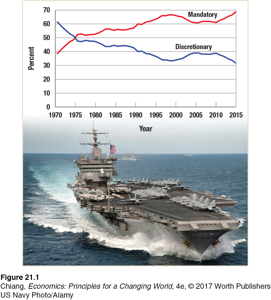
Mandatory spending is authorized by permanent laws and does not go through the same appropriations process as discretionary spending. To change one of the entitlements of mandatory spending, Congress must change the law. Mandatory spending includes such programs as Social Security, Medicare, part of Medicaid, interest on the national debt, and some means-tested income-security programs, including SNAP (Supplementary Nutrition Assistance Program, formerly known as the Food Stamp Program) and TANF (Temporary Assistance to Needy Families). This part of the budget has been growing, as Figure 1 illustrates, and now accounts for over 60% of the budget.

Even though discretionary spending is only 32% of the budget, this is still roughly $1.2 trillion, and the capacity to alter this spending is a powerful force in the economy. Therefore, we are mainly concerned with discretionary spending when we consider fiscal policy.

The exercise of discretionary fiscal policy is done with the express goal of influencing aggregate demand. It involves adjusting government spending and tax policies to move the economy toward full employment, encouraging economic growth, or controlling inflation.

Some examples of the use of discretionary fiscal policy include tax cuts enacted during the Kennedy, Reagan, and George W. Bush administrations. These tax cuts were designed to expand the economy under the belief that people would spend their tax savings, both in the near term and the long run—they were meant to influence both aggregate demand and aggregate supply. Tax increases were enacted under the George H. W. Bush and Clinton administrations in the interest of reducing the government deficit and interest rates. The Roosevelt administration used increased government spending, although small amounts by today’s standards, to mitigate the impact of the Great Depression.

559

Government Spending Although discretionary fiscal policy can get complex, the impact of changes in government spending is relatively simple. As we know, a change in government spending or other components of GDP will cause income and output to rise or fall by the spending change times the multiplier.

This is illustrated in Figure 2 with the economy initially in equilibrium at point e, with real output at Q₀. If government spending increases, shifting aggregate demand from AD₀ to AD₁, aggregate output will increase from Q₀ to Q_f. Because the short-run aggregate supply curve is upward-sloping, some of the increase in output is absorbed by rising prices, reducing the pure spending multiplier discussed in earlier chapters.

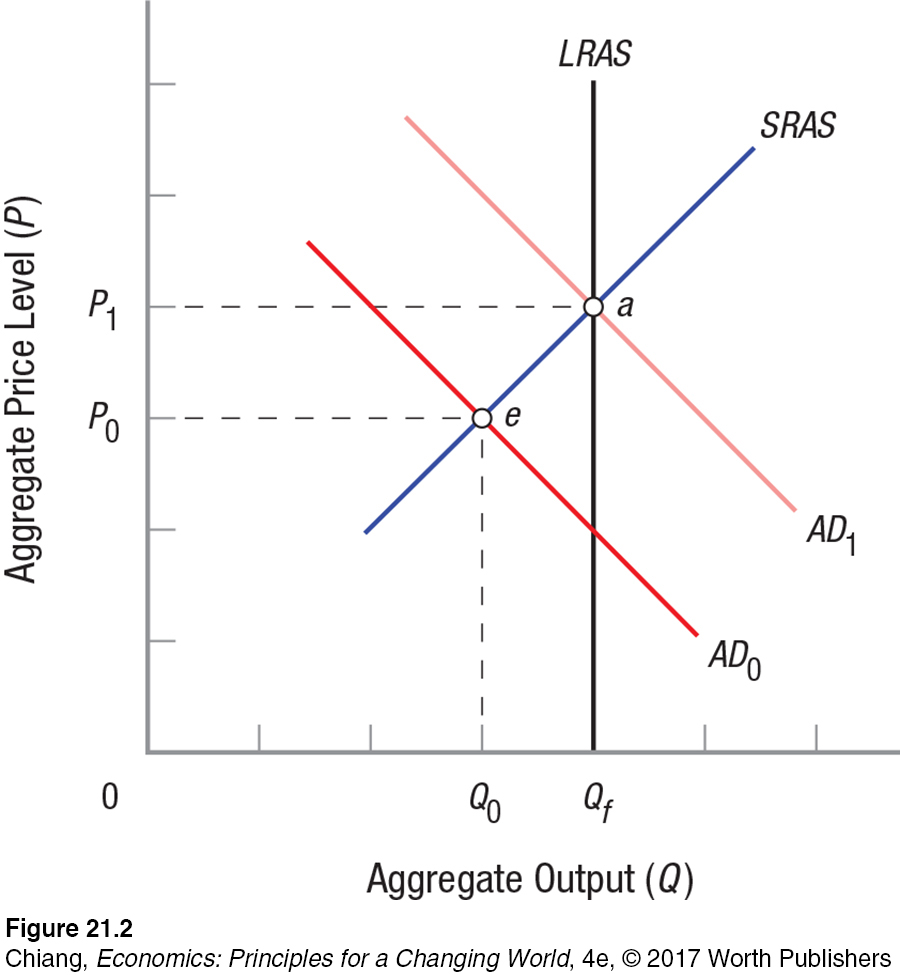
Once the economy reaches full employment (point a), further spending is not multiplied as the economy moves along the LRAS curve, and only higher prices result. Finally, keep in mind that the multiplier works in both directions.

Taxes Changes in government spending modify income by an amount equal to the change in spending times the multiplier. How, then, do changes in taxes affect the economy? The answer is not quite as simple. Let’s begin with a reminder of what constitutes spending equilibrium.

560

When the economy is in equilibrium,

GDP = C + I + G + (X − M)

At equilibrium, all spending injections into the economy equal all withdrawals of spending. To review, injections are activities that increase spending in an economy, such as investment (I), government spending (G), and exports (X). Withdrawals, on the other hand, are activities that remove spending from the economy, such as saving (S), taxes (T), and imports (M). Therefore, in equilibrium:

I + G + X = S + T + M

With this equation in hand, let’s focus on taxes. When taxes are increased, money is withdrawn from the economy’s spending stream. When taxes are reduced, consumers and businesses have more to spend. Disposable income is equal to income minus taxes (Y − T ).

Because taxes represent a withdrawal of spending from the economy, we would expect equilibrium income to fall when a tax is imposed. Consumers pay a tax increase, in part, by reducing their saving. If we initially increase taxes by $100, let’s assume that consumers draw on their savings for $25 of the increase in taxes. Because this $25 in savings was already withdrawn from the economy, only the $75 in reduced spending gets multiplied, reducing the change in income. The reduction in saving of $25 dampens the effect of the tax on equilibrium income because those funds were previously withdrawn from the spending stream. Changing the withdrawal category from saving to taxes does not affect income. A tax decrease has a similar but opposite impact because only the MPC part is spent and multiplied, and the rest is saved and thus withdrawn from the spending stream.

The result is that a tax increase (or decrease, for that matter) has less of a direct impact on income, employment, and output than an equivalent change in government spending. Another way of saying this is that the government tax multiplier is less than the government spending multiplier. Therefore, added government spending leads to a larger increase in GDP when compared to the same reduction in taxes.

Transfers Transfer payments are money payments paid directly to individuals. These include payments for such items as Social Security, unemployment compensation, and welfare. In large measure, they represent our social safety net. We will ignore them as part of the discretionary fiscal policy, because most are paid as a matter of law, but we will see later in the chapter that they are very important as a way of stabilizing the economy.

561

Expansionary fiscal policy involves increasing government spending (such as on highways and education), increasing transfer payments (such as unemployment benefits), and/or decreasing taxes—all to increase aggregate demand. These policies put more money into the hands of consumers and businesses. In theory, these additional funds should lead to higher spending. The precise effect expansionary fiscal policies have, however, depends on whether the economy is at or below full employment.

When the economy is below full employment, an expansionary policy will move the economy to full employment, as Figure 3 shows. The economy begins at equilibrium at point e, below full employment. Expansionary fiscal policy increases aggregate demand from AD₀ to AD₁, and equilibrium output rises to Q_f (point f) as the price level rises to P₁. In this case, one good outcome results—output rises to Q_f—though it is accompanied by one less desirable result, the price level rising to P₁.

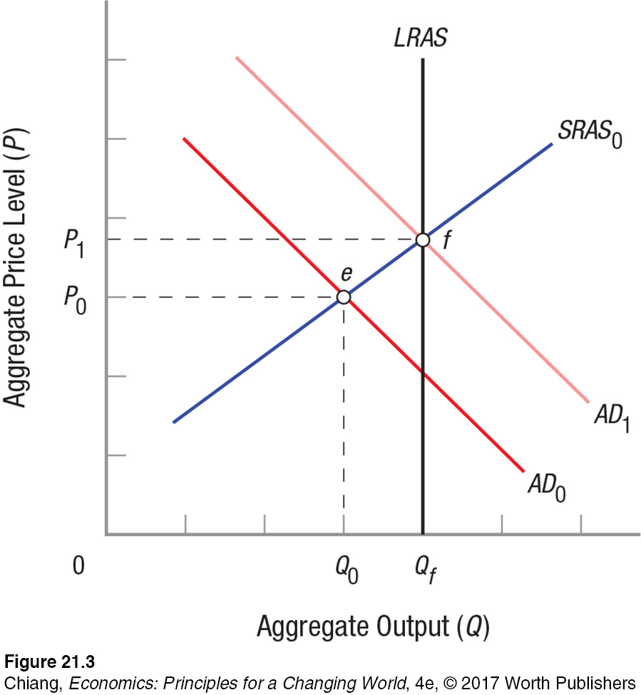
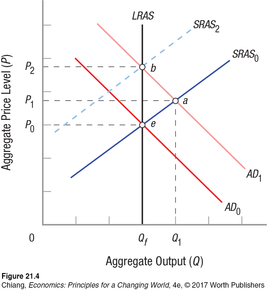
Figure 4 shows what happens when the economy is at full employment. An expansionary policy raises prices without producing any long-run improvement in real GDP. In this figure, the initial equilibrium is already at full employment (point e); therefore, increasing aggregate demand moves the economy to a new output level above full employment (point a), thereby raising prices to P₁. This higher output is only temporary, however, as workers and suppliers adjust their expectations to the higher price level, thus shifting short-run aggregate supply upward to SRAS₂. Short-run aggregate supply declines because workers and other resource suppliers realize that the prices they are paying for products have risen; hence, they demand higher wages or prices for their services. Prices are then pushed up until workers adjust their inflationary expectations and the economy settles into equilibrium at point b. At this point, the economy is again at full employment, but at a higher price level (P₂) than before.

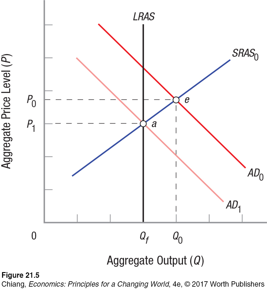
When an economy moves to a point beyond full employment, as just described, economists say an inflationary spiral has set in. The explanation for this phenomenon was suggested earlier. Still, we can already see that one way to reduce such inflationary pressures is to use contractionary fiscal policy. These policies include reducing government spending, reducing transfer payments, and/or raising taxes (increasing withdrawals from the economy). Figure 5 shows the result of contractionary policy. The economy is initially overheating at point e, with output above full employment. Contractionary policy reduces aggregate demand to AD₁, bringing the economy back to full employment at price level P₁ and output Q_f .

562

Exercising demand-side policy requires tradeoffs between increasing output at the expense of raising the price levels, or else lowering price levels by accepting a lower output. When a recession occurs, the public is often happy to trade higher prices for greater employment and output. One would think the opposite would be true when an inflationary spiral loomed on the horizon. Politicians, however, are loath to support contractionary policies that control inflation by reducing aggregate demand, because higher unemployment can cost politicians their jobs. As a result, the demand-side fiscal policy tools—government spending, transfer payments, and taxes—may remain unused. In these instances, politicians often look to the Federal Reserve to use its tools and influence to keep inflation in check. We will examine the Federal Reserve in later chapters.

563