We know by the law of demand that as prices rise, quantity demanded falls. The important question is, How much will quantity demanded fall? Each year, prices for certain items such as college tuition, textbooks, and insurance premiums seem to keep rising, yet very few people stop buying these items. Meanwhile, prices for cable TV and movie theater tickets have also increased, though in these cases many consumers have responded by forgoing these items and looking for alternatives. The concept of elasticity is important in understanding why consumers react more to certain price changes than others.

Price elasticity of demand (E_d) is a measure of how responsive quantity demanded is to a change in price and is defined as

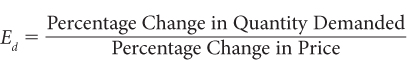
For example, if the price of strawberries increases by 5% and sales fall by 10%, then the price elasticity of demand for strawberries is

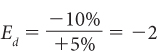
Alternatively, if a 5% reduction in strawberry prices results in a 10% gain in sales, the price elasticity of demand also is 22 (E_d = 10 ÷ [25] 5 22).

Often, we are not given percentage changes. Rather, we are given numerical values and have to convert them into percentage changes. For example, to compute a change in price, take the new price (P_new) and subtract the old price (P_old), then divide this result by the old price (P_old). This approach to calculating percentage changes is known as the base method. Finally, to put this ratio in percentage terms, multiply by 100. In equation form,

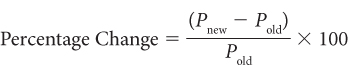
For example, if the old price of gasoline (P_old) was $2.00 per gallon and the new price goes up by $1.00 to $3.00 per gallon, then the percentage change is

The price elasticity of demand is always a negative number. This reflects the fact that the demand curve’s slope is negative: As price increases, quantity demanded falls. Price and quantity demanded stand in an inverse relationship to one another, resulting in a negative value for price elasticity. Economists nevertheless frequently refer to price elasticity of demand in positive terms. They simply use the absolute value of the computed price elasticity of demand. Recalling our examples, where E_d = –2, we can take the absolute value of –2, written as |–2|, and refer to E_d as 2. For price elasticity of demand, we use the absolute value of elasticity and ignore the minus sign.

109

What does this elasticity value of 2 tell us? Quite simply, that for every 1% increase in price, quantity demanded will decline by 2%. Conversely, for every 1% decline in price, quantity demanded will increase by 2%.

Measuring elasticity in percentage terms rather than specific units enables economists to compare the characteristics of various unrelated products. Comparing price and sales changes for houses, cars, and hamburgers in dollar amounts would be so complex as to be meaningless. Because a dollar increase in the price of gasoline is different from a dollar increase in the price of a BMW, by using percentage change, we can compare the sensitivity of demand curves of different products. Percentages allow us to compare changes in prices and sales for any two products, no matter how dissimilar they are; a 100% increase is the same percentage change for any product.

We have seen how to compute the price elasticity of demand, and we have seen why working with percentage changes is so important. Elasticity is a measure giving us a way to compare products with widely different prices and output measures.

All products have some price elasticity of demand. When prices go up, quantity demanded will fall. That is the basis of the negative slope of the demand curve. But people are more responsive to changes in the prices of some products than others. Economists label the demand for goods as being elastic, inelastic, or unitary elastic.

Elastic When the absolute value of the computed price elasticity of demand is greater than 1, economists refer to this as elastic demand. An elastic demand curve is one that is responsive to price changes. At the extreme is the perfectly elastic demand curve shown in panel A of Figure 1. Notice that it is horizontal, showing that the slightest increase in price will result in zero output being sold.

In reality, no branded product—Coca-Cola, Apple iPhone, or Toyota Prius—ever has a perfectly elastic demand curve. Still, products with many close substitutes face highly elastic demand curves. For example, the market for bath tissue is very elastic because nearly all brands—Kleenex, Charmin, Quilted Northern, and others—sell a nearly identical product. If the price of Charmin is raised, sales would quickly fall as people switch to Quilted Northern or Scott. Canned peaches, nuts and bolts, cereal, and bottled water are all examples of products facing highly elastic demands. If one bottled water company were to raise its price, many consumers would switch to other brands, because all bottled water tastes pretty much the same. Demand curves for elastic goods are relatively flat, as shown in panel B in Figure 1.

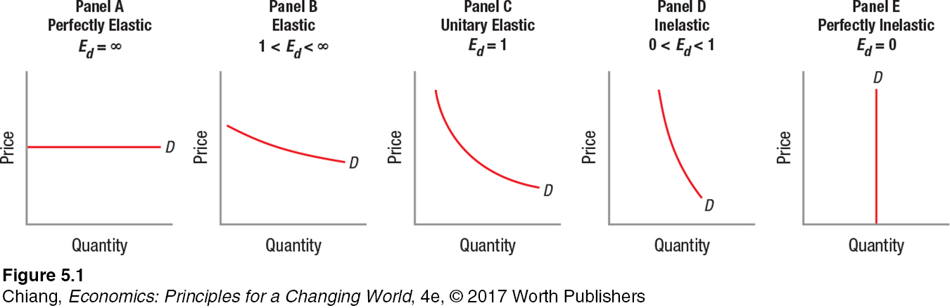
Inelastic At the other extreme, what about products that see little change in sales even when prices change dramatically? The opposite of the perfectly elastic demand curve is the curve showing no response to changes in price. Economists call this a perfectly inelastic demand curve. An example appears in panel E of Figure 1. This curve is vertical, not horizontal as in panel A. For products with perfectly inelastic demands, quantity demanded does not change when price changes.

What products might have inelastic demand? Consider products that are immensely important to our lives but have few substitutes—for example, drugs that treat life-threatening illnesses such as heart disease or stroke, and insulin for diabetics. If people who need these products have the money, they will buy them, no matter how high the price. Some products that are relatively, though not perfectly, inelastic include gasoline, tobacco, and most spices. If gasoline prices rise too sharply, some consumers will curtail their driving. Still, it takes a fairly drastic rise in gasoline prices before most people cut back their driving significantly. Doubling the price of cinnamon will probably not reduce our demand because it is such a small fraction of our overall food budget. Economists define inelastic demand as demand curves with elasticity coefficients that are less than 1. These demand curves are relatively steep, as shown in panel D in Figure 1.

110

Note that the demand for gasoline is inelastic, but the demand for specific brands of gasoline is elastic. Brand preferences for commodities that are nearly identical to one another, such as gasoline, are weak, and many different outlets exist for buying gas. If your local Shell station raises gasoline prices by a significant amount, you will probably go to the Exxon station down the street. Giving up using gasoline altogether, on the other hand, is much harder. Over time, public transportation or electric cars may be possible substitutes for gas-powered cars, but few people will be able to adopt these substitutes in the short run. On the contrary, many people are highly dependent on their gas-powered cars; therefore, gas purchases do not drop substantially when prices rise. Thus, demand for a particular brand of gas (Exxon, Shell) is elastic, while the demand for gasoline as a commodity is inelastic.

Unitary Elastic Elastic demand curves have an elasticity coefficient that is greater than 1, while inelastic demand curves have a coefficient of less than 1. That leaves those products with an elasticity coefficient just equal to 1. Products that meet this condition have unitary elastic demand. This means the percentage change in quantity demanded is precisely equal to the percentage change in price. Panel C of Figure 1 shows a demand curve where price elasticity of demand equals 1. Note that this demand curve is not a straight line. The reasons for this will become clear in our discussion later in the chapter.

Price elasticity of demand measures how sensitive sales are to price changes. But what determines elasticity itself? The four basic determinants of a product’s elasticity of demand are (1) the availability of substitute products, (2) the percentage of income or household budget spent on the product, (3) the difference between luxuries and necessities, and (4) the time period being examined.

111

Substitutability The more close substitutes, or possible alternatives, a product has, the easier it is for consumers to switch to a competing product and the more elastic the demand. For many people, beef and chicken are substitutes, as are competing brands of cola, such as Coke and Pepsi. All have relatively elastic demands. Conversely, if a product has few close substitutes, such as insulin for diabetics or tobacco for heavy smokers, its elasticity of demand tends to be lower.

Proportion of Income Spent on a Product A second determinant of elasticity is the proportion (percentage) of household income spent on a product. In general, the smaller the percent of household income spent on a product, the lower the elasticity of demand. For example, you probably spend little of your income on salt, or on cinnamon or other spices. As a result, a hefty increase in the price of salt, say, 25%, would not affect your salt consumption because the impact on your budget would be tiny. But if a product represents a significant part of household spending, elasticity of demand tends to be greater, or more elastic. A 10% increase in your rent upon renewing your lease, for example, would put a large dent in your budget, significantly reducing your purchasing power for many other products. Such a rent increase would likely lead you to look around for a less expensive apartment.

Luxuries Versus Necessities The third determinant of elasticity is whether the good is considered a luxury or a necessity. Luxuries tend to have demands that are more elastic than those of necessities. Necessities such as food, electricity, and health care are more important to everyday living, and quantity demanded does not change significantly when prices rise. Luxuries such as African safaris, yachts, and designer watches, on the other hand, can be given up when prices rise.

Time Period The fourth determinant of elasticity is the time period under consideration. When consumers have some time to adjust their consumption patterns, demand becomes more elastic. When they have little time to adjust, demand tends to become more inelastic. Thus, as we saw earlier, when gasoline prices rise, most consumers cannot immediately change their transportation patterns; therefore, gasoline sales do not drop significantly. Over time, however, consumers are more likely to make changes, such as buying more fuel-efficient cars.

Table 1 provides a sampling of estimates of elasticities for specific products. As we might expect, medical prescriptions and taxi service have relatively inelastic price elasticities of demand, while foreign travel and restaurant meals have relatively elastic demands.

Source: Compiled from numerous studies reporting estimates for price elasticity of demand.

112

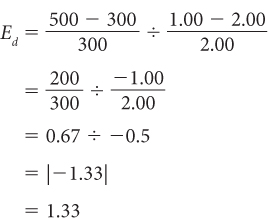
When elasticity is computed between two points, the calculated value will differ depending on whether price is increasing or decreasing. For example, in Figure 2, if the price increases from $1.00 to $2.00, elasticity is equal to

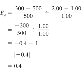
But when price decreases from $2.00 to $1.00, elasticity is equal to

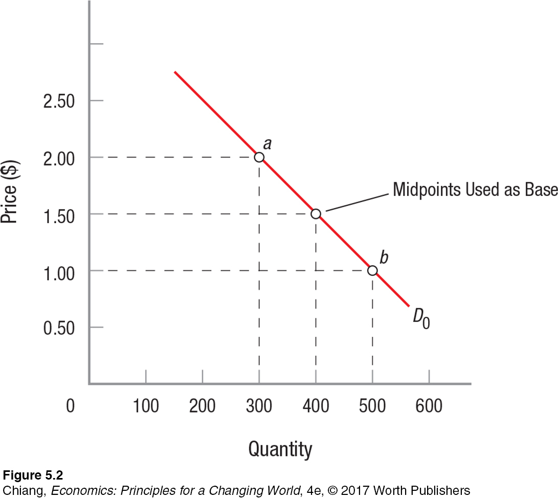
Using Midpoints to Compute Elasticity To avoid getting different results computing elasticity from different directions, economists compute price elasticity using the midpoints of price [(P₀ + P₁)/2] and the midpoints of quantity demanded [(Q₀ + Q₁)/2] as the base. This approach to calculating percentage changes is referred to as the midpoint method.

113

Therefore, the price elasticity of demand formula (assuming price falls from P₀ to P₁ and quantity demanded rises from Q₀ to Q₁) is

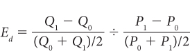
Using the midpoints of price and quantity to compute the relevant percentage changes essentially gives us the average elasticity between point a and point b. Price elasticity of demand is the difference in quantity over the sum of the two quantities divided by 2, divided by the difference in price over the sum of the two prices divided by 2. In Figure 2, the price elasticity of demand between points a and b would equal

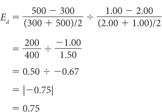
Check for yourself to see that this elasticity formula yields the same results whether you compute elasticity for a price increase from $1.00 to $2.00 or for a price decrease from $2.00 to $1.00.

Now that we have seen what price elasticity of demand is and how to calculate it, let’s put this knowledge to work by looking at how elasticity affects total revenue.

114