162

Indifference curves are a useful device to help us understand consumer demand. Economists use indifference curves, for instance, to shed light on the impact of changes in consumer income and product substitution resulting from a change in product price. Indifference curve analysis, moreover, provides some insight into how households determine their supply of labor (this analysis, however, is left to a later chapter). Before we move on to applications of indifference curve analysis, though, we first need to derive a demand curve from an indifference map.

We derive the demand curve using indifference curve analysis in much the same way we did using marginal utility analysis. Panel A of Figure APX-4 restates the results of Figure APX-3: When you have a budget of $50 per week, the price of pizza is $10, and climbing is $20 per hour, your optimal choice is found at point a. In panel B, we want to plot the demand curve for wall climbing. We know that when wall climbing costs $20 per hour, you will climb for 1.5 hours, so let us indicate this on panel B by marking point a.

163

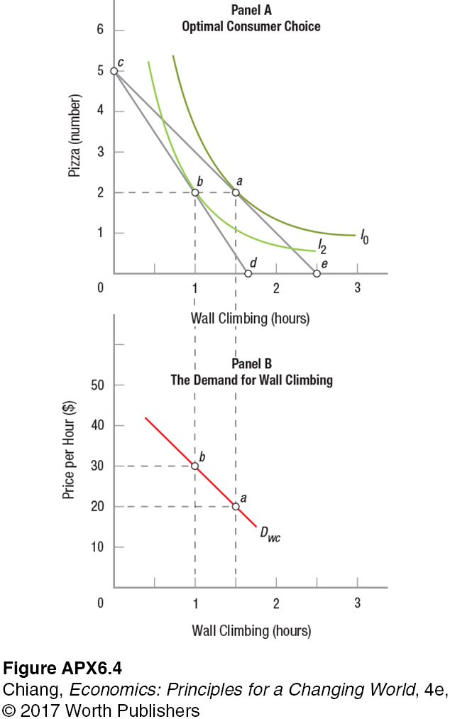
To fill out the demand curve, let us now increase the price of wall climbing to $30 per hour. This produces a new budget line, cd. (Point d is located at 1.67 hours because $50/$30 = 1.67 hours of possible wall climbing.) This shift in the budget line yields a new optimal choice at point b on indifference curve I₂, now indicating the highest level of satisfaction you can attain. As panel A shows, the ultimate result of this hike in the price of wall climbing to $30 an hour is a reduction in your climbing to 1 hour per week. Transferring this result to panel B, we mark point b, where price = $30 and climbing hours = 1. Now connecting points a and b in panel B, we are left with the demand curve for wall climbing.

Once again, therefore, we arrive at the same conclusion using indifference curve analysis as we did earlier using marginal utility analysis. Both approaches are logical and elegant, and both approaches tell us something about the thought processes consumers must use as they make their spending decisions. Indifference curve analysis, however, arrives at its conclusion without requiring that utility be measurable or that consumers perform complex arithmetic computations.

Another way economists use indifference curves is to separate income and substitution effects when product prices change. First, we need to distinguish between these two effects.

When the price of some product you regularly purchase goes up, your spendable income is thereby essentially reduced. If you always buy a latte a day, for instance, and you continue to do so even when the price of lattes goes up, you must then reduce your consumption of other goods. This essentially amounts to a reduction in your income. And we know that when income falls, the consumption of normal goods likewise declines. Hence, when higher prices essentially reduce consumer incomes, the quantity demanded for normal goods generally falls. Economists call this the income effect.

When the price of a particular good rises, meanwhile, the quantity demanded of that good will fall simply because consumers substitute lower-priced goods for it. This is called the substitution effect. Thus, when the price of wall climbing rises from $20 to $30, you cut back on your climbing, in part because you decide to dedicate more of your money to pizza eating. The challenge for us now is to determine just how much of this reduction in your climbing is due to the substitution effect (more pizzas mean less climbing) and how much is due to the income effect (the rise in price effectively leaves you with less money to spend).

Figure APX-5 reproduces panel A of Figure APX-4, adding one line (gh) to divide the total change in purchases into the income and substitution effects. To see how this line is derived, let us begin by reviewing what has happened thus far. At point a, you split your $50 budget into 2 pizzas at $10 each and 1.5 hours of wall climbing at $20 per hour. When the price of wall climbing rose to $30 per hour, you reduced your climbing time to 1 hour.

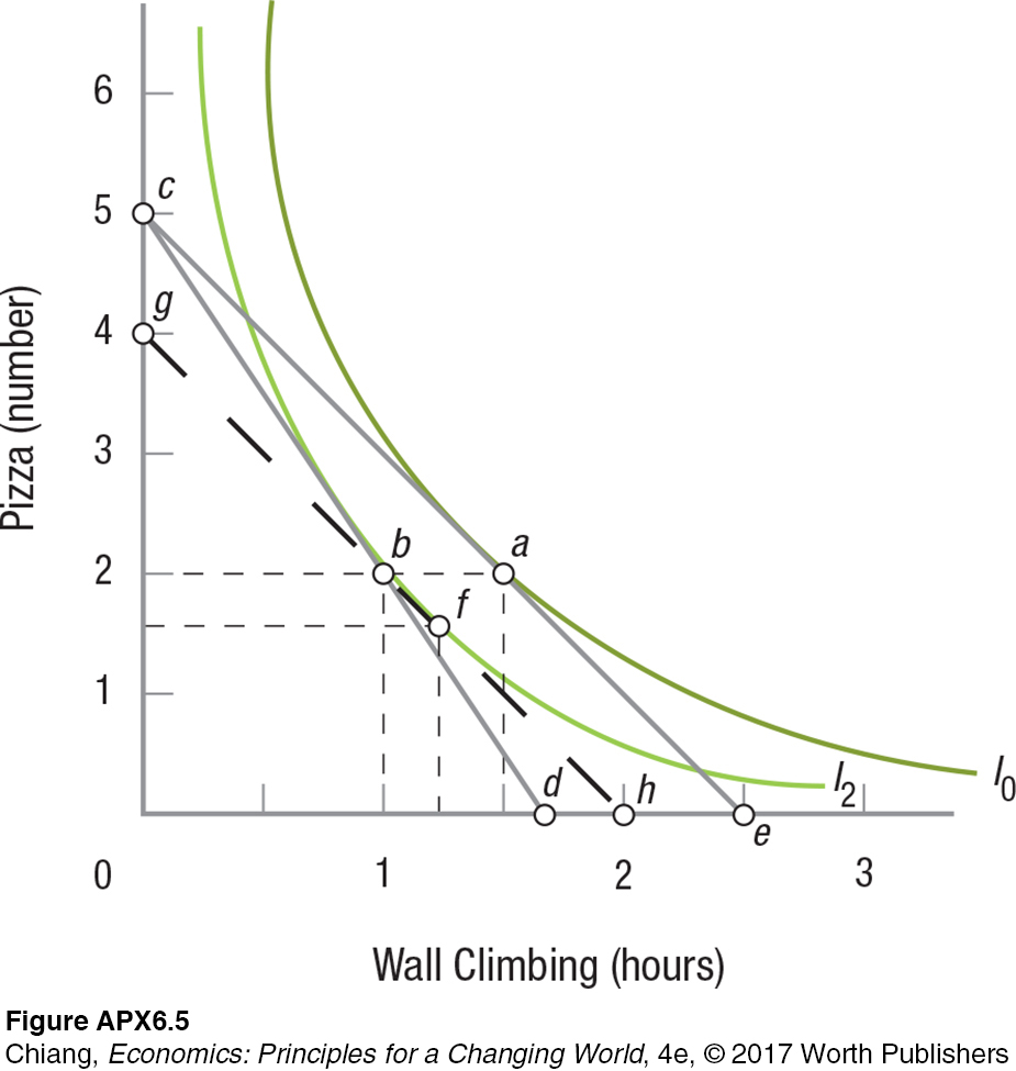
Consider now what happens when we evaluate what you are getting for your current allocation of money, but using the old price of wall climbing ($20 per hour). You are now getting 2 pizzas, worth $10 apiece, plus 1 hour of wall climbing, formerly valued at $20. This means that your budget has effectively been cut to $40. The ultimate effect of the rise in the price of climbing, in other words, has been to reduce your income by $10. In Figure APX-5, the hypothetical budget line gh represents this new budget of $40, though again reflecting the old price of climbing.

Compare the original equilibrium point a on budget line ce with the new equilibrium point f on budget line gh. This new budget line gh reflects a budget of $40 with the old price of climbing ($20 per hour). Had your income previously been $40, you would have reduced your climbing by 15 minutes (to point f). This is the income effect associated with the rise in the price of wall climbing from $20 to $30 per hour. The rising price essentially reduced your income, causing you to consume 15 minutes less of wall climbing and 0.5 fewer pizzas due to this income reduction alone.

The change in price is the only thing that differentiates equilibrium point b from point f, income having been held constant. This difference of 15 minutes between point f and point b therefore represents a substitution effect. By changing the price of climbing while holding income constant, you consume 0.5 more pizza and 15 minutes less wall climbing.

164

Combined, the substitution and income effects constitute the entire change in quantity demanded when the price of wall climbing rises by $10 per hour. The income effect (movement from point a to point f) is a movement from one budget line to another. The substitution effect (movement from point f to point b) is a movement along the new budget line. Together, they represent the total change in quantity demanded. In this case, the income and substitution effects were the same, 15 minutes, but this will not always be the case.

This chapter examined how consumers and households make decisions. Households attempt to maximize their well-being or satisfaction within the constraints of limited incomes. We have seen that the analysis of consumer decisions can be approached in two different ways, using marginal utility analysis or indifference curve analysis.

Marginal utility analysis assumes that consumers can readily measure utility and make complex calculations regarding the utility of various possible consumption choices. Both of these assumptions are empirically rather dubious. This does not, however, invalidate marginal utility analysis; it just makes it difficult to use and test in an empirical context. Indifference curve analysis gives us a more powerful set of analytical tools without these restrictive assumptions.