COSTS OF PRODUCTION
Production tells only part of the story. We have to calculate how much it costs to produce this output in order to figure out if it is profitable to do so. Let’s now bring resource prices, including labor costs, into our analysis to develop the typical cost curves for the firm, both in the short run and the long run.
Short-Run Costs
In a very straightforward way, production costs are determined by the productivity of workers. Ignoring all costs except wages, if you, by yourself, were to produce ten pizzas an hour and you were paid $8 an hour, then each pizza would cost an average of 80 cents to produce—
To understand production costs more generally, we split the production period into the short run and the long run. In the short run, as least one factor is fixed, whereas in the long run, all factors are variable. This has led economists to define costs as fixed and variable.
fixed costs Costs that do not change as a firm’s output expands or contracts, often called overhead. These include items such as lease payments, administrative expenses, property taxes, and insurance premiums.
variable costs Costs that vary with output fluctuations, including expenses such as labor and material costs.
Fixed and Variable Costs Fixed costs are costs that do not change as a firm’s output expands or contracts. Lease or rental payments, administrative overhead, and insurance premiums are examples of fixed costs—
Certain costs don’t always fall so neatly into these two categories. For example, a new wireless communications tower can serve thousands of customers at the same time (and resembles a fixed cost), but once capacity is reached, a new tower is needed (and resembles a variable cost). These types of costs are known as incremental costs. To keep things simple, however, we will assume that all costs fit into either the fixed of variable cost categories, such that total cost (TC) is equal to total fixed cost (FC) plus total variable cost (VC), or
TC = FC + VC
sunk costs Those costs that have been incurred and cannot be recovered.
The measurement of total cost is an important part of determining profits. However, in doing so, sometimes businesses incur costs that are not recoverable should production need to be changed. These irrecoverable costs, which can be both fixed and variable, are called sunk costs, and are incurred by individuals and businesses when making decisions.
Sunk Costs
The previous chapter introduced the concept of sunk costs and how they sometimes lead to imprudent decision making. For example, should you leave in the middle of a movie because it stinks? The cost of the movie ticket has already been paid, and staying until the end might add to the anguish of an already bad situation. Similarly, tuition is a sunk cost. Most colleges and universities do not provide refunds for dropped courses beyond the first week or two of the term.
But what does a “sunk” cost really mean, exactly? Because these costs are not recoverable, future decisions by individuals and businesses should not consider them. For example, the tuition that’s already been paid (the sunk cost) should not influence the decision to drop a course one is failing. Similarly, a business’s decision to air an advertisement on television should not depend on how much it spent producing the ad (the sunk cost), but instead whether the additional cost of airing the ad is justified.
The concept of sunk cost is often difficult to grasp because it goes against what we are often told—

And finally, although most sunk costs are fixed costs, they can also be variable. If one prints 100 party invitations only to find out the party needs to be cancelled, that is an example of a variable sunk cost. The decision to cancel the party shouldn’t depend on the fact that the invitations were already printed.
Now that we have introduced the concepts of fixed, variable, and total cost, let’s discuss how total cost changes when the level of output changes.
Marginal Cost Although measuring total cost is important in determining the overall profitability of a business, the decision of whether to increase or decrease production largely depends on how total costs change when one increases or decreases the quantity produced. If the additional cost of producing one more unit of a good is greater than the additional revenue earned from that unit, then this unit would not be worth producing. Therefore, it is important to measure the change in costs with each additional unit of output produced.
Let’s return to the windsurfing sail business example. Suppose your firm has orders for 10 windsurfing sails this month, and you get an order for 1 more sail at the last minute. Just how much would this additional windsurfing sail cost to produce? Or, in the language of economics, what is the marginal cost of the next sail produced?
marginal cost The change in total costs arising from the production of additional units of output (ΔTC/ΔQ). Because fixed costs do not change with output, marginal costs are the change in variable costs associated with additional production (ΔVC/ΔQ).
Marginal cost is the change in total cost arising from the production of additional units of output. Marginal cost (MC) is equal to the change in total cost (ΔTC) divided by the change in output (ΔQ), or
MC = ΔTC/ΔQ = ΔFC/ΔQ + ΔVC/ΔQ
Note that, for simplicity, we have been discussing changes of 1 unit of output, but we can calculate MC for a change in output of any amount by plugging in the appropriate value for ΔQ. And because fixed costs do not vary with changes in output, ΔFC/ΔQ = 0, and thus marginal cost is also equal to ΔVC/ΔQ.
Table 3 provides us with more complete cost data for your windsurfing sail business. Assuming that you pay $1,000 per month in rent for the warehouse, fixed costs equal $1,000 [column (2)]. Your variable costs (the wages you pay your employees plus the price of raw materials) vary depending on the number of sails produced, and are shown in column (3). The total cost, therefore, is the sum of fixed and variable costs and is shown in column (4). Marginal cost measures the change in total (or variable) cost with each additional sail produced, and is given in column (5).
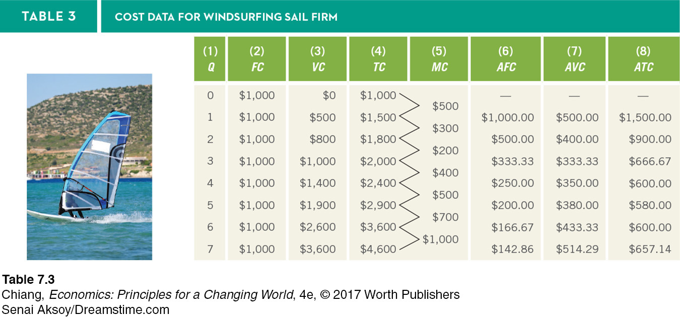
Let’s go through one row so that you can be sure of how we arrived at the numbers in columns (2) to (5). Looking at the row showing 4 sails, the fixed cost is $1,000 because this does not change based on the number of sails produced. Variable cost does change because more work hours are needed to produce more sails; to produce 4 sails, the variable cost is $1,400. Total cost is simply fixed cost plus variable cost, or $2,400 for 4 sails. Finally, the marginal cost of the fourth sail is the change in total cost from producing 3 sails ($2,000) to producing 4 sails ($2,400). Therefore, the marginal cost of the fourth sail is the change from $2,000 to $2,400, or $400, and is shown in column (5) between the third and fourth units. It is common for marginal costs to first fall and then rise, which gives the marginal cost curve its distinct shape, which we will see later.
Average Costs When a firm produces a product or service, it typically wants a breakdown of how much labor, raw material, plant overhead, and sales costs are embedded in each unit of the product. Modern accounting systems permit a detailed breakdown of costs for each unit of production. For our purposes, however, that level of detail is not necessary. For us, cost per unit of output (or average cost), average fixed cost, and average variable cost are sufficient.
If we divide the total cost equation (TC) by total output Q, we get
TC/Q = FC/Q + VC/Q
average fixed cost Equal to total fixed cost divided by output (FC/Q).
average variable cost Equal to total variable cost divided by output (VC/Q).
average total cost Equal to total cost divided by output (TC/Q). Average total cost is also equal to AFC + AVC.
Economists refer to total fixed costs divided by output (FC/Q) as average fixed cost (AFC). This represents the average amount of overhead for each unit of output. Total variable costs divided by output is known as average variable cost (AVC). It represents the labor and raw materials expenses that go into each unit of output. Adding AFC and AVC together results in average total cost (ATC), and thus the preceding equation can be rewritten as
ATC = AFC + AVC
Hence, average cost per unit (ATC) is the sum of average fixed cost (AFC) and average variable cost (AVC).
Average total cost is an important piece of information for firms. Specifically, it provides a general measurement of productivity—
Returning to Table 3, columns (6), (7), and (8) provide the average fixed cost, average variable cost, and average total cost, respectively, for each quantity of windsurfing sails produced. Let’s calculate the average costs of producing 4 sails. The average fixed cost is calculated by taking the fixed cost of $1,000 and dividing it by 4 to equal $250. Average variable cost takes the variable cost of $1,400 and divides by 4 to equal $350 in AVC. We can calculate average total cost in two ways. First, we can take total cost of $2,400 and divide by 4 sails to equal $600 in ATC. Second, we know that ATC = AFC + AVC, so if we know that AFC is $250 and AVC is $350, then $250 + $350 = $600.
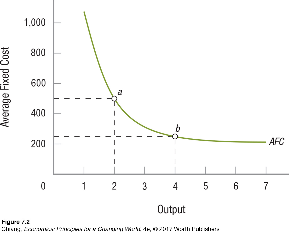
Notice a few trends in the average cost data. First, the average fixed cost falls continuously as more output is produced; this is because your overhead expenses are getting spread out over more and more units of output (this is known as the spreading effect). Figure 2 shows the average fixed cost curve using the data from Table 3. If 2 sails are produced, the average fixed cost is $1,000/2 = $500 (point a on the AFC curve); if 4 sails are produced, the average fixed cost is $1,000/4 = $250 (point b on the AFC curve). Average fixed costs are important to entrepreneurs, who often seek out new businesses with low fixed costs, allowing them to recover these expenses quickly.
Second, average variable costs and average total costs typically fall initially before rising, just like marginal costs. In the short run, these costs initially fall as the costs of procuring variable inputs fall and due to the spreading effect (which affects the average total cost curve), but these costs eventually rise with greater output as access to available resources dries up, leading to diminishing returns (resulting in a diminishing returns effect). Finally, average variable cost will always be smaller than the average total cost according to the ATC = AFC + AVC equation. These trends will be important as we make greater use of average cost in the next three chapters.
Short-Run Cost Curves for Profit-Maximizing Decisions
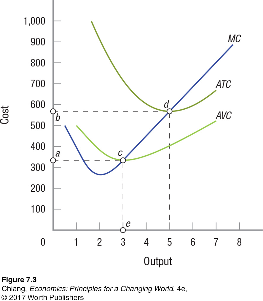
Table 3 provides the numerical values for costs. Although all of the costs are important in their own way, we focus on three costs that will provide guidance to firms in their need to maximize profits. These are average variable cost, average total cost, and marginal cost. Let us now translate these costs into figures to make their analysis simpler. Figure 3 shows the three cost measures in graphical form, drawn using the data from Table 3.
Average Variable Cost (AVC) The AVC and ATC curves are U-
In Figure 3, the average variable cost curve reaches its minimum where 3 sails are produced (point c). Since AVC = VC/Q, then VC = AVC × Q. Thus, at point c, VC is equal to the rectangular area 0ace, or $1,000 ($333.33 × 3).
Average Total Cost (ATC) Average total cost equals total costs divided by output (ATC = TC/Q), or average fixed costs plus average variable cost (ATC = AFC + AVC). In Figure 3, the average total cost reaches its minimum where 5 sails are produced (point d). At this point, the average total cost is $580. As in the previous example, we can calculate the total cost of the firm at any point along the average total cost curve by multiplying the average total cost by the output produced. For example, the total cost of 5 sails would be $580 × 5 = $2,900, exactly as shown in Table 3.
Therefore, the use of cost curves allows us to determine both the total and average costs for a firm, which again are important components in determining profits. Still, we cannot proceed until we examine marginal costs, a key determinant in whether firms should produce more or less output.
Marginal Cost (MC) Drawing our discussion of short-
Notice that the marginal cost curve intersects the minimum points of both the AVC and ATC curves. This is not a coincidence. Marginal cost is the cost necessary to produce another unit of a given product. When the cost to produce another unit is less than the average of the previous units produced, average costs will fall. For the AVC curve in Figure 3, this happens at all output levels less than 3 units (point c); for the ATC curve, it happens at all output levels less than 5 units (point d). But when the cost to produce another unit exceeds the average cost for all previous output, average costs will rise.
In Figure 3, this happens at output levels greater than 3 units (point c) for AVC and greater than 5 units (point d) for ATC. Over these ranges, marginal cost exceeds AVC and ATC, respectively, and thus the two curves rise. At points c and d, marginal cost is precisely equal to average variable cost and average total cost, respectively, and thus the AVC and ATC curves are at their minimum values (where the slopes are zero).
The average variable cost, average total cost, and marginal cost curves will help us analyze the profit-
We have now examined short-
Long-Run Costs
In the long run, firms can adjust all factor inputs (such as labor and capital) to meet the needs of the market. Here, we focus on variations in plant size, while recognizing that all other factors, including technology, can vary.
Figure 4 shows the short-
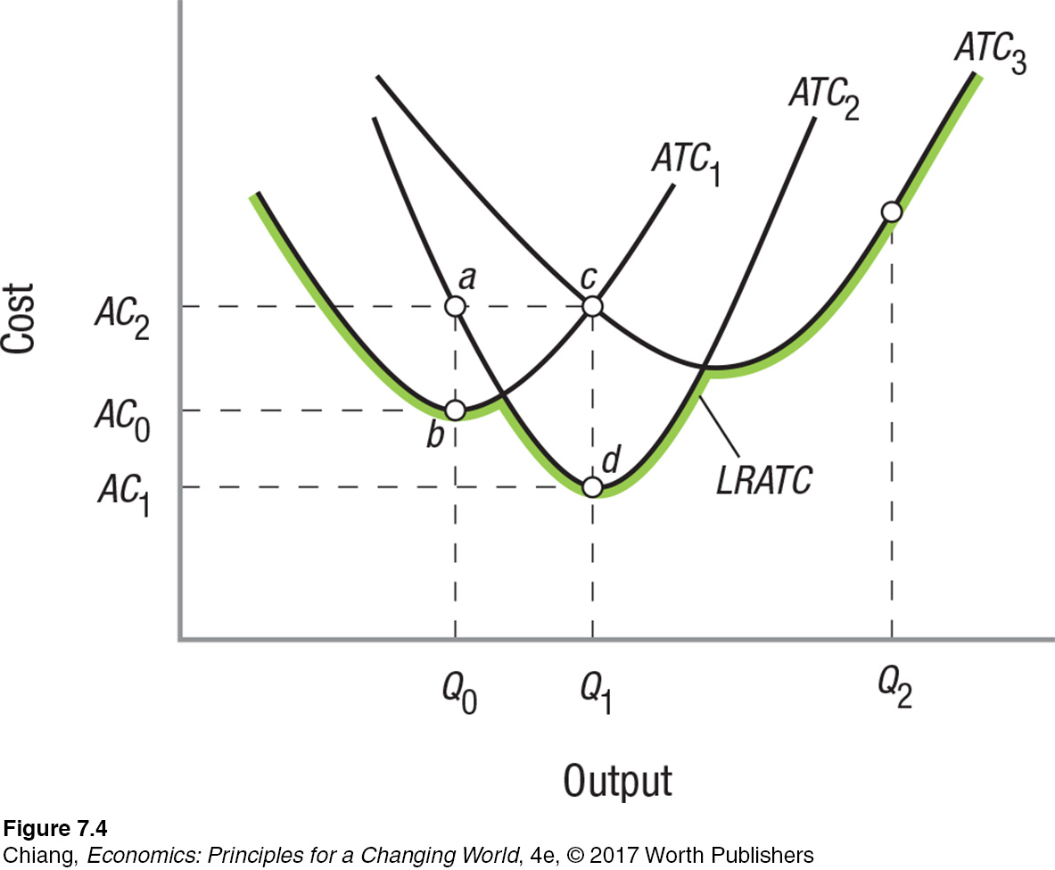
Therefore, at lower levels of production, plant 1 is able to achieve the lowest average cost. However, plant 2 and plant 3 achieve greater cost savings at higher levels of production. Once output rises to Q1, plant 2 begins to enjoy the benefits of a lower average cost of production. The additional machines mean that plant 2 can produce Q1 for AC1 (point d), whereas the machines in plant 1 become overwhelmed at this level of output, resulting in an average cost of AC2 (point c). Similarly, if a firm expects market demand eventually to reach Q2, it would want to build plant 3 because plant 1 and plant 2 are too small to accommodate that level of production efficiently.
long-
Long-
Although the LRATC curve in Figure 4 is relatively bumpy, it will tend to smooth out as more plant size options are considered. In some industries, such as agriculture and food service, the options for plant size and production methods are virtually unlimited. In other industries, such as semiconductors, however, sophisticated plants may cost several billion dollars to build and require being run at near capacity to be cost-
These huge, sophisticated plants are so complex that Intel Corporation has dedicated teams of engineers that build new plants and operate them exactly as all others. These teams ensure that any new plant is a virtual clone of the firm’s other operating facilities. Even small deviations from this standard have proven disastrous to cost control in the past.
economies of scale As a firm’s output increases, its LRATC tends to decline. This results from specialization of labor and management, and potentially a better use of capital and complementary production techniques.
Economies and Diseconomies of Scale As a firm’s output increases, its LRATC tends to decrease. This is because, as the firm grows in size, economies of scale result from such items as specialization of labor and management, better use of capital, and increased possibilities for making several products that utilize complementary production techniques.
A larger firm’s ability to have workers specialize in particular tasks reduces the costs associated with shifting workers from one task to another. Similarly, management in larger operations can use technologies and specialized capital equipment that smaller firms cannot afford because of their smaller production volumes. Therefore, larger firms are better able to engage in complementary production and use by-
The area for economies of scale is shown in Figure 5 at levels of output below Q0 (average costs are falling).
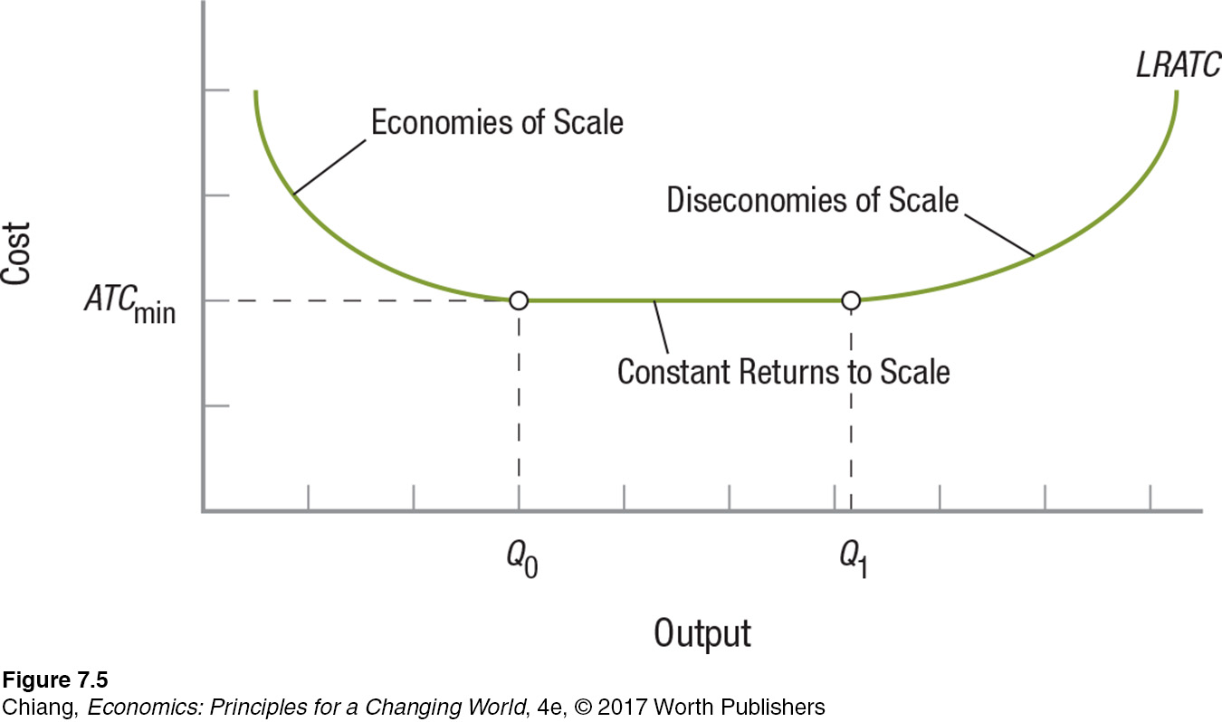
constant returns to scale A range of output where average total costs are relatively constant. The expansion of fast-
In many industries, there is a wide range of output wherein average total costs are relatively constant. Examples include fast-
diseconomies of scale A range of output where average total costs tend to increase. Firms often become so big that management becomes bureaucratic and unable to control its operations efficiently.
As firms continue to grow, they eventually encounter diseconomies of scale. At some point, the firm gets so big that management is unable to control its operations efficiently. Some firms become so big that they get bogged down in bureaucracy and cannot make decisions quickly. In the late 1980s, Apple fell into this trap—
economies of scope By producing a number of products that are interdependent, firms are able to produce and market these goods at lower costs.
Economies of Scope When firms produce a number of products, it is often cheaper for them to produce another product when the production processes are interdependent. These economies are called economies of scope. For example, once a company has established a marketing department, it can take on the campaign of a new product at a lower cost. It has already developed the expertise and contacts necessary to sell the product. Book publishers can introduce a new book into the market more quickly and cheaply, and with more success than can a new firm starting in the business.
Some firms generate ideas for products, then send the production overseas. After they have been through this process, they become more efficient at it. Economists refer to this as learning by doing. Economies of scope often play a role in mergers as firms look for other firms with complementary products and skills.
Procter & Gamble makes hundreds of household products, taking advantage of large economies of scope by producing many products that use the same inputs and equipment. For example, some of the chemicals used to produce Tide detergent are also used to produce Cascade dishwasher tablets.
Role of Technology We know that technology creates products that were the domain of science fiction writers of the past. Dick Tracy’s wrist radio, first introduced in the comics of 1940s, has now morphed into the many wireless products we see today.

But we should mention in passing the role technology plays in altering the shape of the LRATC curve. The output level at which diseconomies of scale are reached has significantly and continuously expanded since the beginning of the Industrial Revolution.
Enhanced production techniques, instantaneous global communication, and the use of computers in accounting and cost control are just a few recent examples of ways in which technology has permitted firms to increase their scale beyond what anyone had imagined possible 50 years earlier. Who would have imagined a century ago that one firm could have millions of employees and billions of dollars in annual sales? Today, Walmart has more than 2 million employees and annual sales of over $500 billion.
What spurs firms and entrepreneurs to develop new technologies and bring new products to market? Three things: profits, profits, and profits. In this chapter, we analyzed where profits come from by looking at what firms do, how they measure profits, and how they determine production and costs. In the next chapter, we will look at revenues, as well as examine how firms can maximize their profits by adjusting output to market demand.

Live Like a Royal: Castles Turning into Hotels
Why did investors in Ireland spend enormous sums of money to convert historic castles and homes into hotels?
As global demand for tourism rises, travelers are increasingly seeking unique experiences that they cannot have at home. For example, with the popularity of shows such as Downton Abbey, who wouldn’t want to live the life of nobility, even if just for a day? One industry that has been eager to provide such experiences to travelers is the hospitality industry. Hotels have long attempted to offer unique amenities to their guests. But can hotels go one step further by offering a history lesson and a chance for an ordinary person to ape nobility?
In Ireland, a country with many historical landmarks and castles, hoteliers have transformed historical homes and even centuries-

At Dromoland Castle near Shannon, Ireland, guests enter the grounds of a refurbished 16th-
GO TO  TO PRACTICE THE ECONOMIC CONCEPTS IN THIS STORY
CHECKPOINT
COSTS OF PRODUCTION
Fixed costs (overhead) are those costs that do not vary with output, including lease payments and insurance. Fixed costs occur in the short run—
in the long run, firms can change plant size or even exit an industry. Variable costs rise and fall as a firm produces more or less output. These variable costs include raw materials, labor, and utilities.
Total cost equals fixed cost plus variable cost (TC = FC + VC).
Average fixed cost, average variable cost, and average total cost provide a general measure of efficiency when looking at the total amount of output produced.
Marginal cost is the change in total cost divided by the change in output (MC = DTC/DQ). Marginal cost provides important information to firms deciding whether to produce more or less output.
The long-
run average total cost curve (LRATC) represents the lowest unit cost at which specific output can be produced in the long run. As a firm grows in size, economies of scale result from specialization of labor and better use of capital, while diseconomies of scale occur because a firm gets so big that management loses control of its operations and the firm becomes bogged down in bureaucracy.
Economies of scope result when firms produce a number of interdependent products, so it is cheaper for them to add another product to the line.
Modern communications and computers have permitted firms to become huge before diseconomies of scale are reached.
QUESTION: In the late 1990s, Boeing reported that it took roughly 12 years and $15 billion to bring a new aircraft from the design stage to a test flight. Boeing signed a 20-
Answers to the Checkpoint questions can be found at the end of this chapter.
This immense $15 billion development cost is a fixed cost that is spread over more planes as production rises. Therefore, Boeing has an incentive to enter into contracts with airlines to ensure that both economies of scale and economies of scope can be achieved.