Suppose you find a rare comic book on eBay that you believe is worth $100, and start putting in bids hoping to buy it. After a week, you get the comic book with the winning bid of $80. You are happy because not only will you get the comic book you’ve been looking for, but you have also paid a price lower than what you were willing to pay. However, you’re likely not the only one who is happy. The person who sold you that comic book found it in her granddad’s old trunk that she inherited, and had hoped to get at least $60 for it. In fact, she ended up receiving more money than the minimum amount she had hoped to receive. In this situation, the transaction took place, and both the buyer and seller are better off.

When consumers go about their everyday shopping or when they seek out their next major purchase, their objective typically is to find the lowest price relative to the perceived value of the product. It is the reason why consumers compare prices, shop online, or bargain with sellers. In other words, the general goal of consumers is to find the product at a price no greater than their willingness-to-pay (perceived value); if the price is less, consumers benefit more. These “savings,” so to speak, are referred to as consumer surplus, and are a measure of the net benefits consumers receive in the market.

Producers also have a corresponding objective. When an entrepreneur opens up a new business, her intention is to maximize its success by getting the highest price for a product relative to its cost for as large a quantity as possible. Sometimes this is achieved by selling fewer units at a higher markup (such as rare art), while other times it is achieved through the sale of mass quantities of products at relatively small markups (such as goods sold at Walmart). Regardless of the strategy used, the general goal of producers is to obtain a price at least equal to their willingness-to-sell; if the price is higher, producers benefit more. These gains are called producer surplus, and are a measure of the net benefits producers receive in the market.

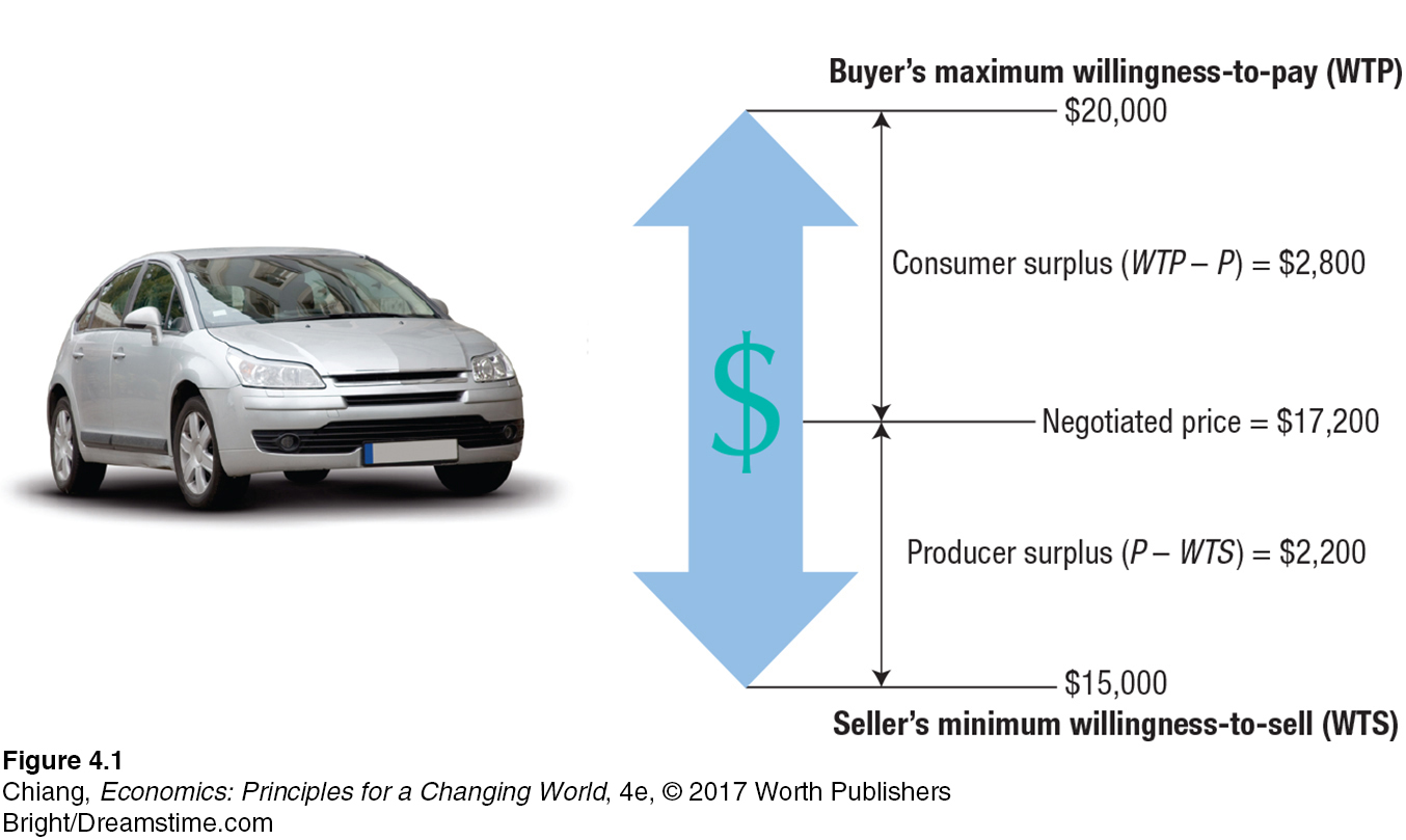
Now that you have an intuitive sense of what consumer surplus and producer surplus are, let’s look more carefully into how they are measured. We begin with a single case of a buyer and a seller at a car dealership. Suppose you are the buyer, and you find a car that interests you. Let’s assume that the most you would be willing to pay for that car is $20,000. In other words, you find the car to be worth $20,000, but paying that price would be the worst-case scenario other than not buying the car at all. You would rather get a better deal by negotiating with the sales manager. But now let’s look at the other side: Assume that the sales manager has a minimum price of $15,000 at which he is willing to sell the car. Selling the car at this price would be his worst-case scenario other than not selling the car.

87

We have now determined a potential “gain” of $5,000 that can be shared by the buyer and seller depending on the final negotiated price for this car. Figure 1 shows this gain as the difference between the buyer’s willingness-to-pay (WTP) and the seller’s willingness-to-sell (WTS). Assume that the final negotiated price of the car is $17,200. We can now use this information to calculate consumer surplus (WTP – P = $20,000 – $17,200 = $2,800) and producer surplus (P – WTS = $17,200 – $15,000 = $2,200).

This example is unique in that the price of the car is negotiated between the buyer and seller. In most of our daily transactions, however, the prices of goods and services are not negotiated. When you go to the grocery store, all of the prices are fixed. You don’t negotiate over the price of milk, bread, or chicken. Nonetheless, the measurements of consumer surplus and producer surplus remain the same when prices are fixed.

Suppose that instead of just one buyer and one seller, the market contains dozens or even thousands of buyers and sellers. What would change? Let’s look at the market for Frisbees used in the popular intramural sport of Ultimate. First, each of the many buyers would have a different WTP, which would be represented as a downward-sloping demand curve (by definition, demand is just a collection of WTPs of all consumers in a market). Second, each of the many sellers would have a different WTS, which would be represented as an upward-sloping supply curve. But the definition of consumer surplus (WTP – P) and producer surplus (P – WTS) remains the same, except that now we apply it to the entire market. Figure 2 illustrates how consumer and producer surplus is determined in a small market for Frisbees with specific consumers and firms and for the overall market.

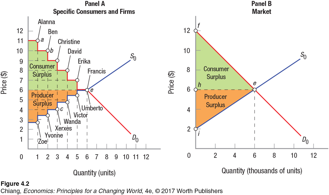
Panel A in Figure 2 represents a small market with 6 individual buyers and 6 individual sellers, with an equilibrium price of $6 (from equilibrium point e) at which 6 units of output are sold. In this market, Alanna has the highest willingness to pay, because she values a Frisbee to be worth $11. Because the market determines that $6 is the price everyone pays, Alanna clearly gets a bargain by purchasing the unit and receiving a consumer surplus equal to $5 ($11 – $6). Ben, however, values a Frisbee a little less at $10, but still receives a consumer surplus of $4 ($10 – $6). And so on for Christine, David, and Erika, who receive a consumer surplus of $3, $2, and $1, respectively. Only Francis, who values a Frisbee to be worth exactly the same amount as the market price, earns no consumer surplus. Total consumer surplus for the 6 consumers in panel A is found by adding all of the individual consumer surpluses for each unit purchased. Thus, total consumer surplus in panel A is equal to $5 + $4 + $3 + $2 + $1 + $0 = $15.

88

In a similar way, assume that each point on the supply curve represents a specific seller, each with a Frisbee to sell but each with a different willingness to sell. Equilibrium price is still $6; therefore, Zoe, who is willing to sell her Frisbee for just $2.67, receives a producer surplus of $3.33 ($6 – $2.67). Yvonne, Xerxes, Wanda, and Victor, who each have a higher willingness-to-sell, receive a correspondingly smaller producer surplus equal to $2.67, $2.00, $1.33, and $0.67, respectively. And Umberto, who had a willingness-to-sell of $6, receives no producer surplus for his sale. Total producer surplus in panel A is equal to $3.33 + $2.67 + $2.00 + $1.33 + $0.67 + $0 = $10.

Panel B illustrates consumer and producer surplus for an entire market. For convenience, we have assumed that the market is 1,000 times larger than that shown in panel A, so the x axis is output in thousands. Whereas in panel A we had discrete buyers and sellers, we now have one big market; therefore, consumer surplus is equal to the area under the demand curve and above equilibrium price, or the area of the shaded triangle labeled “consumer surplus.”

To put a number to the consumer surplus triangle (feh) in panel B, we can compute the area of the triangle using the formula 1/2(base × height). Thus, total market consumer surplus in panel B is [1/2 × (6,000) × ($12 – $6)] = $18,000. The shaded triangle labeled “producer surplus” (area hei) is found in the same way by computing the value of the triangle. Producer surplus is equal to [1/2 × (6,000) × ($6 – $2)] = $12,000.

Although we simplify the calculation of consumer and producer surplus using the area of the triangle, remember that it is still the sum of many individual consumer and producer surpluses. It is merely because of the fact that markets have thousands of buyers and sellers that the steps in panel A of Figure 2 become very small, thus resulting in smooth demand and supply curves in panel B.

We have now defined consumer surplus and producer surplus for individuals and for markets. But how do we know whether the market leads to an ideal outcome for consumers and producers? The next section goes on to reveal the efficiency of markets.

89