COMPETITIVE LABOR DEMAND
demand for labor Demand for labor is derived from the demand for the firm’s product and the productivity of labor.
The competitive firm’s demand for labor is derived from the demand for the firm’s product and the productive capabilities of a unit of labor.
Marginal Revenue Product
marginal physical product of labor The additional output a firm receives from employing an added unit of labor (MPPL = ΔQ ÷ ΔL).
marginal revenue product The value of another worker to the firm is equal to the marginal physical product of labor (MPPL) times marginal revenue (MR).
Assume that a firm wants to hire an additional worker, and that worker is able to produce 15 units of the firm’s product. This additional output a firm receives from employing an added unit of labor is the marginal physical product of labor (MPPL), calculated as the change in output divided by the change in labor, or ΔQ ÷ ΔL. Further, assume that the product sells in a competitive market for $10 a unit, and labor is the only input cost (such as blackberry picking in Oregon). The last worker hired is therefore worth $150 to the firm (15 × $10 = $150). The value of another worker to the firm is referred to as the marginal revenue product (MRPL), and is equal to the marginal physical product of labor times marginal revenue:
MRPL = MPPL × MR
If the cost of hiring this worker is $150 or less (assuming that a normal profit is included in the cost of labor), then the firm will hire this person. If the wage rate for labor exceeds $150, a competitive firm will not hire this marginal worker.
MRPL differs from worker to worker. As we saw in a previous chapter, production is subject to diminishing marginal returns. In the example of blackberry picking, the first blackberry picker takes the nearest low-
To see how this works in greater detail, look at Table 1. The production function here is similar to the one used earlier in the chapter on production. Column (1) is labor input (L), column (2) is total output (Q), and column (3) is the MPPL.
In this example, the firm is operating in a competitive market; therefore, it can sell all the output it produces at the prevailing market price of $10. When a fourth worker is added, output is increased from 25 to 40, resulting in a marginal physical product of labor of 15 units. Multiplying 15 units times the marginal revenue—
value of the marginal product The value of the marginal product of labor (VMPL) is equal to marginal physical product of labor times price, or MPPL × P.
A related term to marginal revenue product is the value of the marginal product, defined as VMPL = MPPL × P. Because competitive firms are price takers for whom marginal revenue is equal to the price of the product (MR = P), VMPL = MRPL in the competitive case.
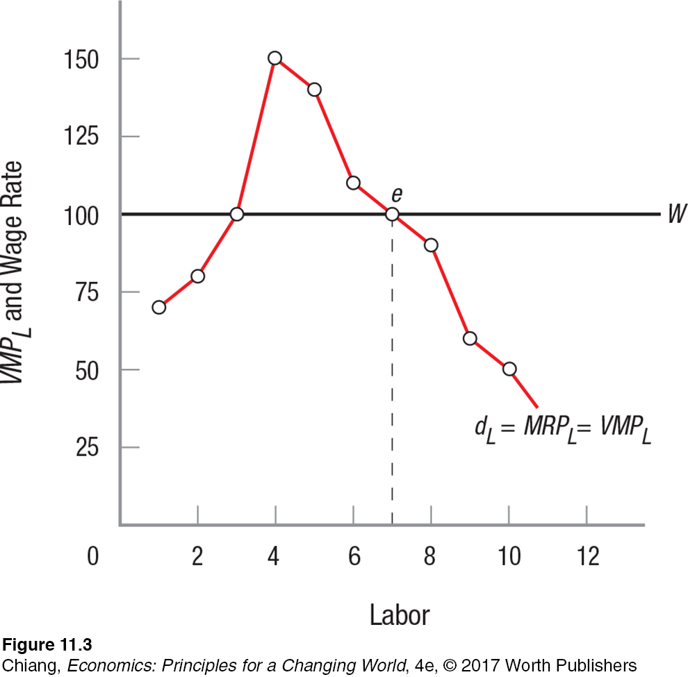
Column (4) contains the firm’s MRPL. Additional workers add this value to the firm. Thus, the marginal revenue product curve is the firm’s demand for labor, which is graphed in Figure 3. Note how the marginal revenue product reaches a maximum at 4 workers, as shown in column (4) of the table and in the figure.
Competitive firms hire labor from competitive labor markets. Because each firm is too small to affect the larger market, it can hire all the labor it wants at the market-
Table 1 and Figure 3 assume that the going wage for labor (W) is $100. For our firm, this results in 7 workers being hired at $100 (point e), because this is the employment level at which W = MRPL. Note that W = MRPL at 3 workers as well, but because the marginal revenue product is greater than the wage rate for workers 4 to 6, the firm would hire 7 workers, not 3, to maximize its gains. The value to the firm of hiring the seventh worker is just equal to what the firm must pay this worker. Profits are maximized for the competitive firm when workers are hired out to the point at which MRPL = W.
| TABLE 1 | COMPETITIVE LABOR MARKET | |||
| (1) L | (2) Q | (3) MPPL | (4) MRPL (P = $10) | (5) W |
| 0 | 0 | — | — | — |
| 1 | 7 | 7 | $70 | $100 |
| 2 | 15 | 8 | $80 | $100 |
| 3 | 25 | 10 | $100 | $100 |
| 4 | 40 | 15 | $150 | $100 |
| 5 | 54 | 14 | $140 | $100 |
| 6 | 65 | 11 | $110 | $100 |
| 7 | 75 | 10 | $100 | $100 |
| 8 | 84 | 9 | $90 | $100 |
| 9 | 90 | 6 | $60 | $100 |
| 10 | 95 | 5 | $50 | $100 |
However, if market wages were to fall to $90, the firm would hire an eighth worker to maximize profits, because with 8 employees, MRPL is also equal to $90.
In a competitive labor market, the prevailing wage ($90 in this case) would be paid to each worker regardless of the actual MRPL. Thus, firms maximize gains from hiring workers in the labor market similarly to how consumers maximize consumer surplus when buying goods and services in the product market.
Factors That Change Labor Demand
The demand for labor is derived from product demand and labor productivity—
Changes in Product Demand A decline in the demand for a firm’s product will lead to lower market prices, reducing MRPL, and vice versa. As MRPL for all workers declines, labor demand will shift to the left. Anything that changes the price of the product in competitive markets will shift the firm’s demand for labor.
Over the past 5 years, the movie industry has changed as people now primarily download movies directly to their tablets instead of purchasing or renting DVDs. This has decreased demand for movies on DVDs, and subsequently led to a reduction in prices. As a result, labor demand by DVD movie manufacturers has shifted to the left.

Changes in Productivity Changes in worker productivity (usually increases) can come about from improving technology or because a firm uses more capital or land along with its workforce. For example, some supermarkets have introduced digital price tags on their store shelves, allowing prices to be changed remotely instead of having a store clerk physically replace each tag on the shelf as prices change. Such improvements in productivity raise MPPL. The demand for the marginal worker rises, shifting the demand for labor to the right as firms are willing to pay higher wages. To be sure, the number of workers hired may fall due to digitalization, but the workers programming the price codes, as in any capital-
Changes in the Prices of Other Inputs Changes in input prices can affect the demand for labor through their effect on capital prices. For example, rising steel and glass prices can dramatically raise the costs of equipment such that firms are unable to replace aging equipment. Without the ability to afford the rising costs of new capital equipment, firms are forced to use more labor in place of capital, thus increasing the demand for labor. Relative costs of capital and labor will therefore affect the capital and labor mix firms choose for their production.
At this point, we know that more labor will be hired when wages fall, but how much more? The answer depends on the elasticity of demand for labor.
Elasticity of Demand for Labor
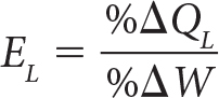
elasticity of demand for labor The percentage change in the quantity of labor demanded divided by the percentage change in the wage rate.
The elasticity of demand for labor (EL) is the percentage change in the quantity of labor demanded (QL) divided by the percentage change in the wage rate (W). This elasticity is found the same way we calculated the price elasticity of demand for products, except that the wage rate instead of the price of the product is used in the denominator.
The elasticity of demand for labor measures how responsive the quantity of labor demanded is to changes in wages. An inelastic demand for labor is one in which the absolute value of the elasticity is less than 1. Conversely, an elastic curve’s computed elasticity is greater than 1.
The time firms have to adjust to changing wages will affect elasticity. In the short run, when labor is the only truly variable factor of production, elasticity of demand for labor is more inelastic. In the long run, when all production factors can be adjusted, elasticity of demand for labor tends to be more elastic.
Factors That Affect the Elasticity of Demand for Labor
Although time affects elasticity, three other factors also affect the elasticity of demand for labor: elasticity of product demand, ease of substituting other inputs, and labor’s share of the production costs. Let’s briefly consider each of these.
Elasticity of Demand for the Product The more price elastic the demand for a product, the greater the elasticity of demand for labor. Higher wages result in higher product prices, and the more easily consumers can substitute away from the firm’s product, the greater the number of workers who will become unemployed. An elastic demand for labor means that employment is more responsive to wage rates. The opposite is true for products with inelastic demands.
Ease of Input Substitutability The more difficult it is to substitute capital for labor, the more inelastic the demand for labor will be. At this point, computers cannot yet substitute for pilots in commercial airplanes, which results in an inelastic demand for pilots. As a result, pilots have been able to secure high wages from airlines. The easier it is to substitute capital for labor, the less bargaining power workers have, and labor demand tends to be more elastic.
Labor’s Share of Total Production Costs The share of total costs associated with labor is another factor determining the elasticity of demand for labor. If labor’s share of total costs is small, the demand for labor will tend to be rather inelastic. In the example of airline pilots, the percentage of costs going to pilot wages is small, perhaps 10%. Thus, a large increase in pilot wages would have a relatively small effect on ticket prices and demand, resulting in little change in demand for pilot labor. The opposite is true when labor’s share of costs is large.
Competitive Labor Market Equilibrium
Generalized market equilibrium in competitive labor markets requires that we take into account the industry supply and demand for labor. The market supply for labor (SL) is the horizontal sum of the individual labor supply curves in the market.
The market demand for labor, however, is not simply a summation of the demand for labor by all the firms in the market. When wages fall, for instance, this affects all firms—
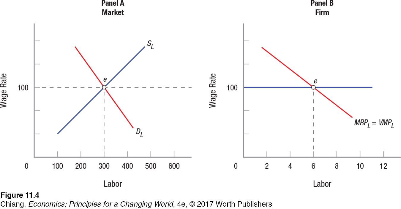
Turning to Figure 4, we have put both sides of the market together. In panel A, the competitive labor market determines equilibrium wage ($100 per day) and employment (300 workers) based on market supply and demand. Individual firms, in light of their own situation, hire 6 workers at the point where this equilibrium wage is equal to marginal revenue product (MRPL), point e in panel B. Much like the product markets we discussed in earlier chapters, the invisible hand of the marketplace sets wages and in the end determines employment.
To this point, we have assumed that labor markets are competitive and that firms are able to hire as many workers as they desire at the prevailing wage rate. This analysis of competitive labor markets goes a long way, but just as with product markets, it does not tell the whole story. We are going to look at two familiar cases in which the competitive model is clearly not the case. The first case is economic discrimination in the labor market in which the personal preferences of employers, employees, or consumers cause some workers to be preferred over others, creating wage differentials. The second case involves unions, which restrict labor supply in certain industries to raise wages relative to nonunion industries. When wage differentials exist for workers performing the same tasks, we say that labor markets are imperfect. There are other, more technical instances of imperfect labor markets—

Life as a Sherpa: Risking One’s Life in Exchange for Financial Security
Why do the Sherpa people of Nepal risk their lives performing hard manual labor for tourists at very meager pay?
In the Himalayas, home to nine of the ten tallest mountains on the planet, mountaineers come from around the world to conquer one of the peaks that dot the landscape. Kathmandu, the capital of Nepal, is the starting point for many of these mountaineers who range from seasoned climbers seeking to conquer the tallest peak on every continent, to the “leisure” climber allured to the Himalayas in search of a life story. But behind the scenes of these great expeditions is an ethnic group critical to the mountaineering industry: Sherpas.
How essential are Sherpas to the existence of this industry?

Sherpas are a Nepalese ethnic group who for generations have served as porters, guides, and technical specialists to foreign climbers. Sherpas have lived in the Himalayas for centuries, developing an ability to handle high-
The labor market for mountaineering support has high demand. Most climbers spend $50,000 or more on a 2-
As long as wages can adjust for risks such as those Sherpas face every day, one person’s nightmare job might be another person’s dream job.
GO TO  TO PRACTICE THE ECONOMIC CONCEPTS IN THIS STORY
CHECKPOINT
COMPETITIVE LABOR DEMAND
The firm’s demand for labor is a derived demand—
derived from consumer demand for the product and the productivity of labor. Marginal revenue product is equal to the marginal physical product of labor times marginal revenue.
The demand for labor is equal to the marginal revenue product of labor for competitive firms.
The demand for labor curve will change if there is a change in the demand for the product, if there is a change in labor productivity, or if there is a change in the price of other inputs.
The elasticity of demand for labor is equal to the percentage change in quantity of labor demanded divided by the percentage change in the wage rate.
The elasticity of demand for labor will be more elastic the greater the elasticity of demand for the product, the easier it is to substitute other factors for labor, and the larger the share of total production costs attributed to labor.
Market equilibrium occurs at the point at which the labor demand and supply curves intersect.
QUESTIONS: Individuals are different in terms of ability, attitude, and willingness to work. Given this fact, does it make sense to assume labor is homogeneous? Does this model better fit firms such as Walmart that hire 800+ employees at each store at roughly standardized wages than, say, firms such as Google, which look for highly skilled computer geeks?
Answers to the Checkpoint questions can be found at the end of this chapter.
For many jobs, firms have standardized procedures that each employee follows. Therefore, the difference in productivity between individuals is relatively narrow. While homogeneous labor is a simplification, taking in everyone’s difference would make analysis impractical. No, the model explains both since markets exist for each broad category of workers.