chiangmicro4e

Nonlinear Relationships

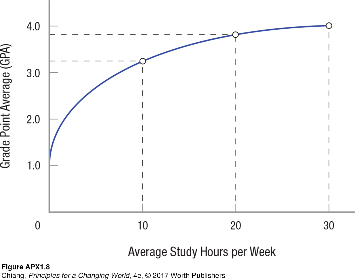
It would be nice for model builders if all relationships were linear, but that is not the case. It is probably not really the case with the amount of studying and GPA either. Figure APX-8 depicts a more realistic nonlinear and positive relationship between studying and GPA. Again, we assume that one can get a D average (1.0) without studying and reach a maximum of straight A’s (4.0) with 30 hours of studying per week.

Figure 1.8: FIGURE APX-8 STUDYING AND YOUR GPA (NONLINEAR)

Figure 1.8: This nonlinear graph of study hours and GPA is probably more typical than the one shown in Figures APX-6 and APX-7. Like many other things, studying exhibits diminishing returns. The first hours of studying result in greater improvements to GPAs than further hours of studying.

Figure APX-8 suggests that the first few hours of study per week are more important to raising GPA than are the others. The first 10 hours of studying yield more than the last 10 hours. The first 10 hours of study raise one’s GPA from 1.0 to 3.3 (a gain of 2.3), while the 20th to the 30th hours raise GPA from 3.8 to 4.0 (a gain of only 0.2). This curve exhibits what economists call diminishing returns. Just as the first bite of pizza tastes better than the 100th, so the first 5 hours of studying bring a bigger jump in GPA than the 25th to 30th hours.

Computing the Slope of a Nonlinear Curve

As you might suspect, computing the slope of a nonlinear curve is a little more complex than for a linear line. But it is not that much more difficult. In fact, we use essentially the same rise over run approach that is used for linear lines.

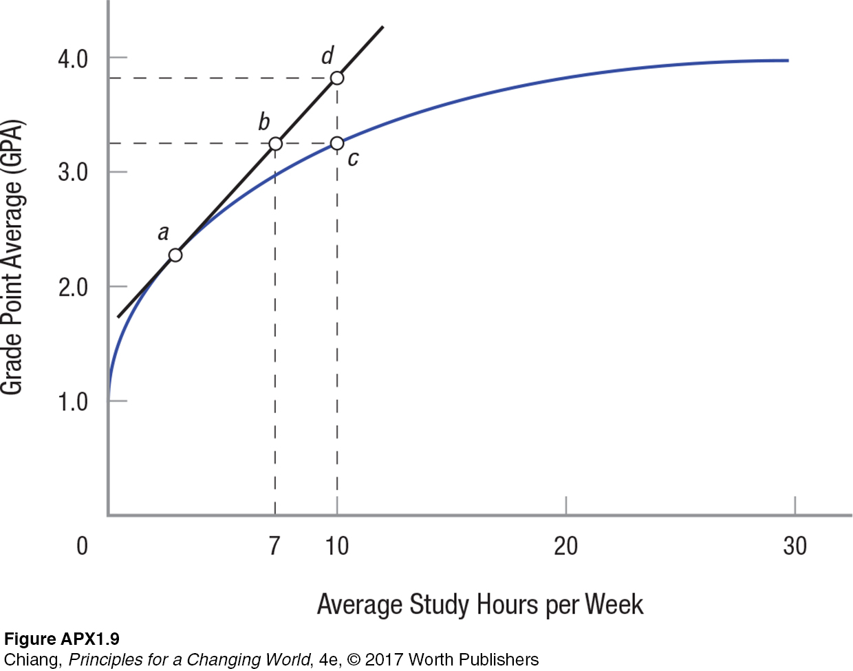
Looking at the curve in Figure APX-8, it should be clear that the slope varies for each point on the curve. It starts out very steep, then begins to level out above 20 hours of studying. Figure APX-9 shows how to compute the slope at any point on the curve.

Figure 1.9: FIGURE APX-9 COMPUTING SLOPE FOR A NONLINEAR CURVE

Figure 1.9: Computing the slope of a nonlinear curve requires that you compute the slope of each point on the curve. This is done by computing the slope of a tangent to each point.

Computing the slope at point a requires drawing a line tangent to that point, then computing the slope of that line. For point a, the slope of the line tangent to it is found by computing rise over run again. In this case, it is length dc ÷ bc or [(3.8 – 3.3) ÷ (10 – 7)] = 0.5 ÷ 3 = 0.167. Notice that this slope is significantly larger than the original linear relationship of 0.1. If we were to compute the slope near 30 hours of studying, it would approach zero (the slope of a horizontal line is zero).