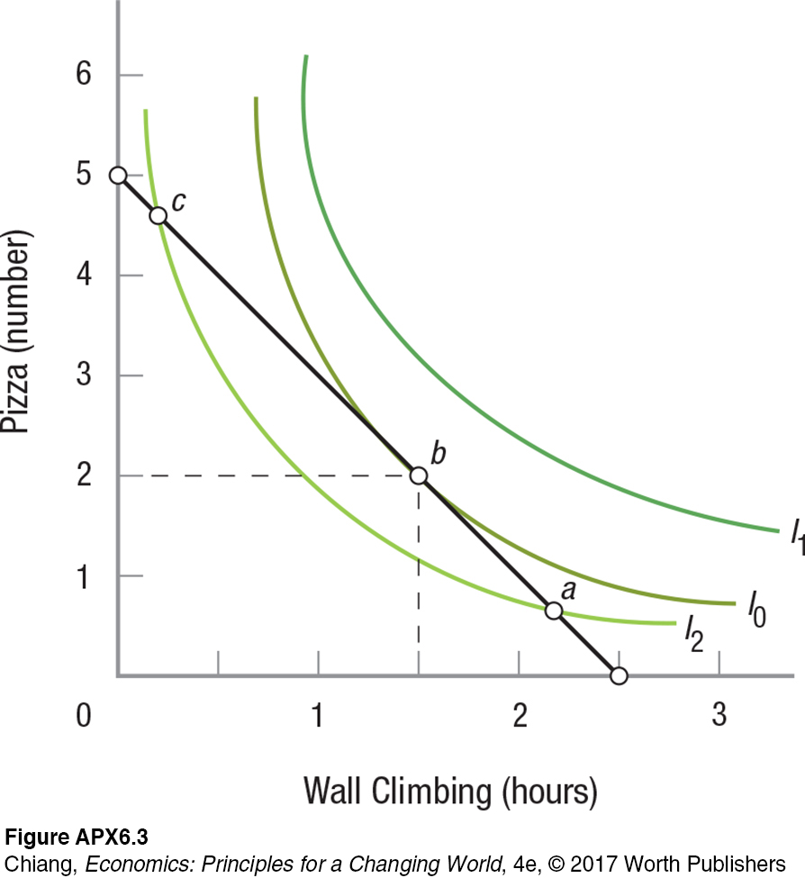
Figure APX-3 superimposes a budget line of $50 per week onto a preference map that assumes pizzas cost $10 each and wall climbing costs $20 per hour. Maximizing your satisfaction on your limited income requires that you purchase some bundle of goods on the highest possible indifference curve. In this example, the best you can do is indicated by point b: 2 pizzas and 1.5 hours of wall climbing. Clearly, if you were to pick any other point on the budget line, your satisfaction would be diminished because you would end up on a lower indifference curve (such as points a or c on I₂ in Figure APX-3). It follows that the indifference curve running tangent to the budget line identifies your best option—in this case, the indifference curve that just touches the budget line at point b.

Of course, this is the same result we reached earlier using marginal utility analysis, specifically in Table 2. Notice, however, that using indifference curve analysis, we did not have to assume that utility can be measured. We were able to understand how you would allocate your budget between two goods so as to achieve the highest possible level of satisfaction, even without knowing exactly how high that level might be.