PERFECT COMPETITION: SHORT-RUN DECISIONS
Figure 1 in the previous section presented a perfectly competitive market with an equilibrium price of $200. This translates into a horizontal demand curve for individual firms at that price. Individual firms are price takers in this competitive situation: They can sell as many units of their product as they wish at $200 each.
Marginal Revenue
marginal revenue The change in total revenue from selling an additional unit of output. Because competitive firms are price takers, P = MR for competitive firms.
Economists define marginal revenue as the change in total revenue that results from the sale of one additional unit of a product. Marginal revenue (MR) is equal to the change in total revenue (ΔTR) divided by the change in quantity sold (Δq); thus,
MR = ΔTR/Δq
Total revenue (TR), meanwhile, is equal to price per unit (p) times quantity sold (q); thus,
TR = p × q
In a perfectly competitive market, we know that price will not change based on the output of any one firm. And because marginal revenue is defined as the change in revenue that comes from selling 1 more unit, marginal revenue is simply equal to price. To verify, suppose a firm sells 10 units of a good at $200 each, earning a total revenue of $2,000. If the firm sells 11 units at $200 each, total revenue becomes $2,200. Using our marginal revenue equation, the added revenue a firm receives from selling the 11th unit is $200, which is equal to the product price. Thus, determining marginal revenue in a perfectly competitive market is easy. As we will see in later chapters, this gets more complicated in market structures in which firms have some control over price.
Profit-Maximizing Output
Suppose that you own a windsurfing sail manufacturing firm in a perfectly competitive market. Figure 2 shows the price and marginal cost curve that your firm faces while it seeks to maximize profits. As the price and cost curve show, you can sell all you want at $200 a sail. Our first instinct might be to conclude that you will produce all that you can, but this is not the case. Given the marginal cost curve shown in Figure 2, if you produce 85 units, profit will be less than the maximum possible. This is because revenue from the sale is $200, but the 85th sail costs $210 to produce (point b). This means producing this last sail reduces profits by $10.
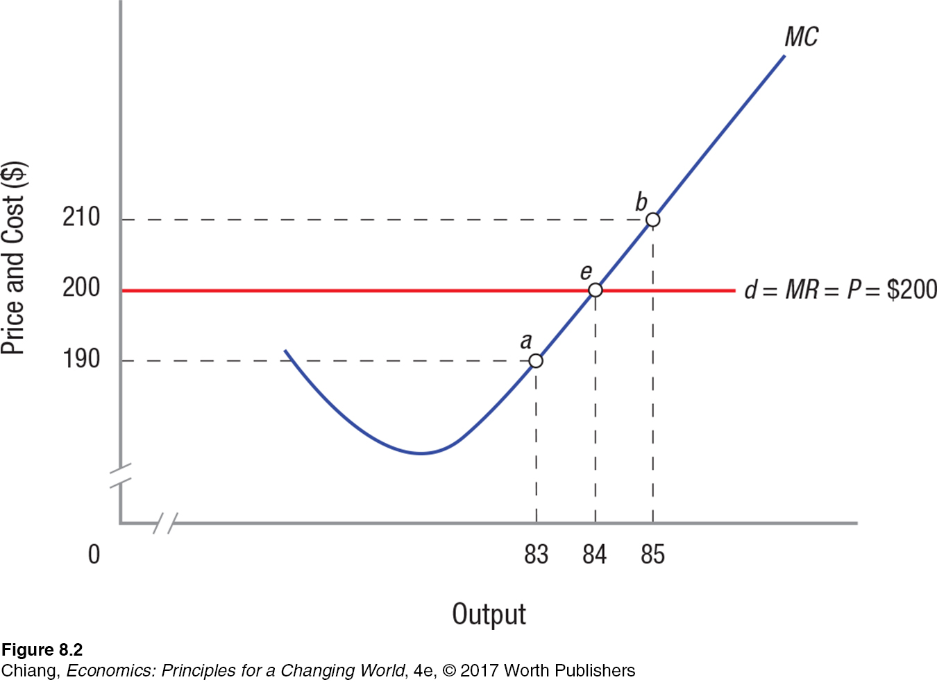
Suppose instead that you produce 84 sails. The revenue from selling the 84th unit (MR) is $200. This is precisely equal to the added cost (MC) of producing this unit, $200 (point e). Therefore, your firm earns zero economic profit by producing and selling the 84th sail. Zero economic profit, or normal profits, mean that your firm is earning a normal return on its capital by selling this 84th sail. If you produce only 83 sails, however, the additional cost (point a) will be less than the price, and you will have to relinquish the normal return associated with the 84th sail. Profits from selling 83 sails will therefore be lower than if 84 sails are sold because the normal return on the 84th sail is lost.
profit-
These observations lead us to a profit-
Economic Profits
Continuing with the example of your windsurfing sail manufacturing firm, assume that the market has established a price of $200 for each sail. Your marginal revenue and cost curves are shown in Figure 3 (the MR and MC curves are the same as those shown in Figure 2).
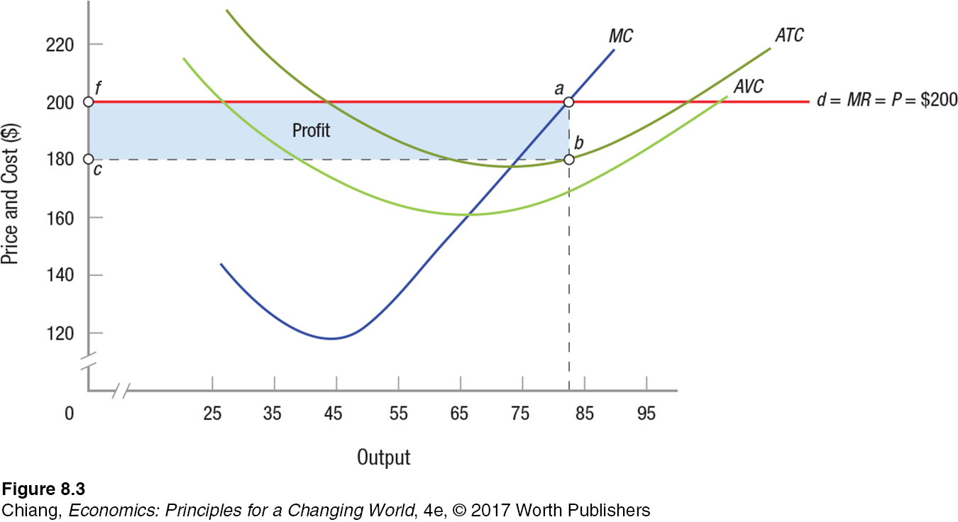
Earlier, we found that profits are maximized when your firm is producing output such that MR = MC, in this case, 84 sails. Looking at Figure 3, we see that profits are maximized at point a, because this is where MR = MC at $200. We can compute the profit in this scenario by multiplying average profit (profit per unit) by output. Average profit equals price minus average total cost (P − ATC). In the figure, the average total cost of producing 84 sails is $180 (point b). Thus, when 84 sails are produced, average profit is the distance ab in Figure 3, or $200 − $180 = $20. Total profit, or average profit times output [(P − ATC) × Q], is $20 × 84 = $1,680; this is represented in the figure by area cfab. This area also is equivalent to total revenue minus total cost (TR − TC).
Note that there is a profit-
Five Steps to Maximizing Profit
Profit maximization is an important goal of any firm in any market structure. Yet, understanding revenue and cost curves can be frustrating given the many market structures and the different types of curves facing each market. Wouldn’t it be useful to have a single approach when solving for a profit-
Let’s review how we solved for the profit-
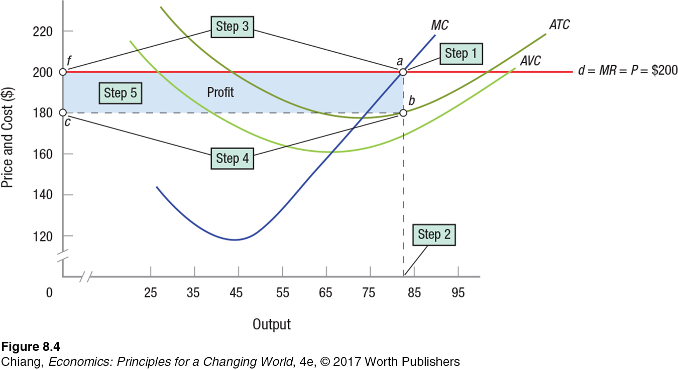
Step 1: Find the point at which marginal revenue (MR) equals marginal cost (MC). Remember that in a perfectly competitive market, MR equals price.
Step 2: At the point at which MR = MC, find the corresponding point on the horizontal axis; this is the profit-
Step 3: At the profit-
Step 4: Again using the profit-
Step 5: Find the profit, which is the rectangle formed between the profit-
Some of these steps might seem redundant. However, using this approach will help you to identify the profit-
Normal Profits
When the price of a windsurfing sail is $200, your firm earns economic profits. Consider what happens, however, when the market price falls to $175 a sail. This price happens to be the minimum point on the average total cost curve, corresponding to an output of 75 sails. Figure 5 shows that at the price of $175, the firm’s demand curve is just tangent to the minimum point on the ATC curve (point e), which means that the distance between points a and b in Figure 3 has shrunk to zero. By producing 75 sails, your firm earns normal profits, or zero economic profit.
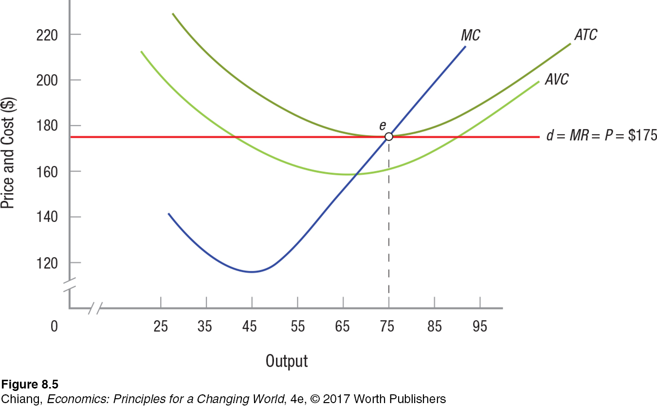
normal profits Equal to zero economic profits; where P = ATC
Remember that when a firm earns zero economic profit, it is generating just enough income to keep investor capital in the business. When the typical firm in an industry is earning normal profits, there are no pressures for firms to enter or leave the industry. As we will see in the next section, this is an important outcome in the long run.
Loss Minimization and Plant Shutdown
Assume for a moment that an especially calm summer with little wind leads to a decline in the demand for windsurfing sails. Assume also that, as a consequence, the price of windsurfing sails falls to $170. Figure 6 illustrates the impact on your firm. Market price has fallen below your average total cost of production (which takes into account the fixed cost, which in this case is $1,000, an amount determined in the previous chapter), but remains above your average variable cost. Profit maximization—
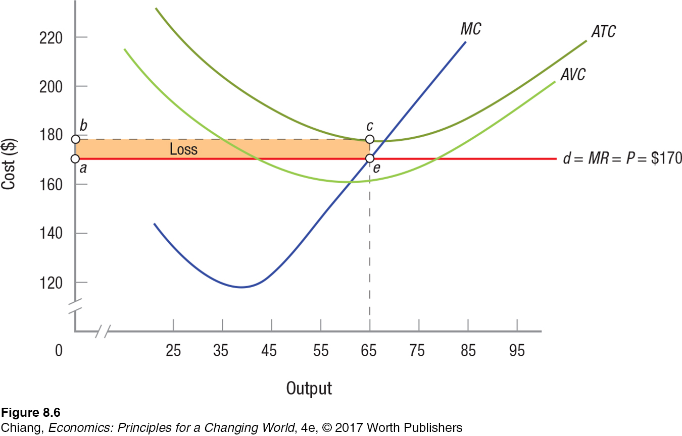
Using Figure 6, at 65 units, the average total cost at this production level is $178; thus, with a market price of $170, loss per unit is $8. The total loss on 65 units is $8 × 65 = $520, corresponding to area abce.
These results may look grim, but consider your alternatives. If you were to produce more or fewer sails, your losses would just mount. You could, for instance, furlough your employees. But you will still have to pay your fixed costs of $1,000. Without revenue, your losses would be $1,000. Therefore, it is better to produce and sell 65 sails, taking a loss of $520, thereby cutting your losses nearly in half.
shutdown point When price in the short run falls below the minimum point on the AVC curve, the firm will minimize losses by closing its doors and stopping production. Because P < AVC, the firm’s variable costs are not covered; therefore, by shutting the plant, losses are reduced to fixed costs only.
But what happens if the price of windsurfing sails falls to $160? Such a scenario is shown in Figure 7. Your revenue from the sale of sails has fallen to a level just equal to variable costs. If you produce and sell 60 units of output (where MR = MC), you will be able to pay your employees their wages, but have nothing left over to pay your overhead; thus, your loss will be $1,000. Point e in Figure 7 represents a shutdown point, because your firm will be indifferent to whether it operates or shuts down—
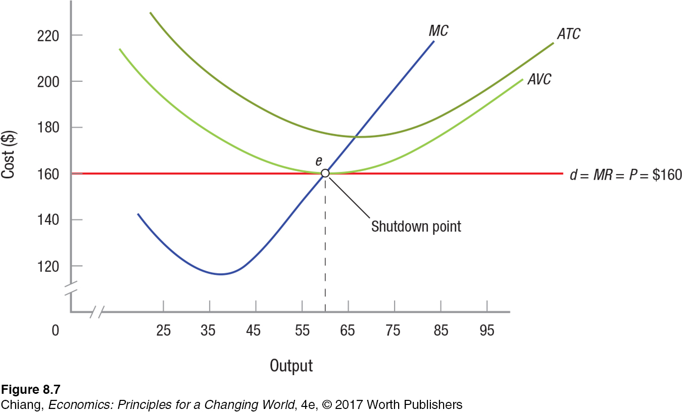
If prices continue to fall below $160 a sail, your losses will grow still further, because revenue will not even cover wages and other variable expenses. Once prices drop below the minimum point on the AVC curve (point e in Figure 7), losses will exceed total fixed costs and your loss-
How practical is it to shut down production? That depends on the size of the firm and whether short-
HERBERT SIMON (1916–2001)
NOBEL PRIZE
When he was awarded the Nobel Prize for Economics in 1978, Herbert Simon (1916–
In his book Administrative Behavior, Simon approached economics and the behavior of firms from his outsider’s perspective. Simon thought real-
To Simon, the reality is not that firms tilt at the mythical windmill of maximizing profits, but that, as he said in his Nobel Prize acceptance speech, they recognize their limitations and instead try to come up with an “acceptable solution to acute problems” by setting realistic goals and making reasonable assessments of their successes or failures.
Simon’s views provided a new approach to analyzing market structure models. Simon brought data, theories, and knowledge from other disciplines and paved the way for behavioral economics (discussed in Chapter 6) to eventually become a prominent field of economics by broadening its scope and applying more realistic conditions found in the marketplace.
The Short-Run Supply Curve
A glance at Figure 8 will help to summarize what we have learned so far. As we have seen, when a competitive firm is presented with a market price of P0, corresponding to the minimum point on the AVC curve, the firm will produce output of q0. If prices should fall below P0, the firm will shut its doors and produce nothing. If, on the other hand, prices should rise to P1, the firm will sell q1 and earn normal profits (zero economic profits). And if prices continue climbing above P1, say, to P2, the firm will earn economic profits by selling q2. In each instance, the firm produces and sells output where MR = MC.
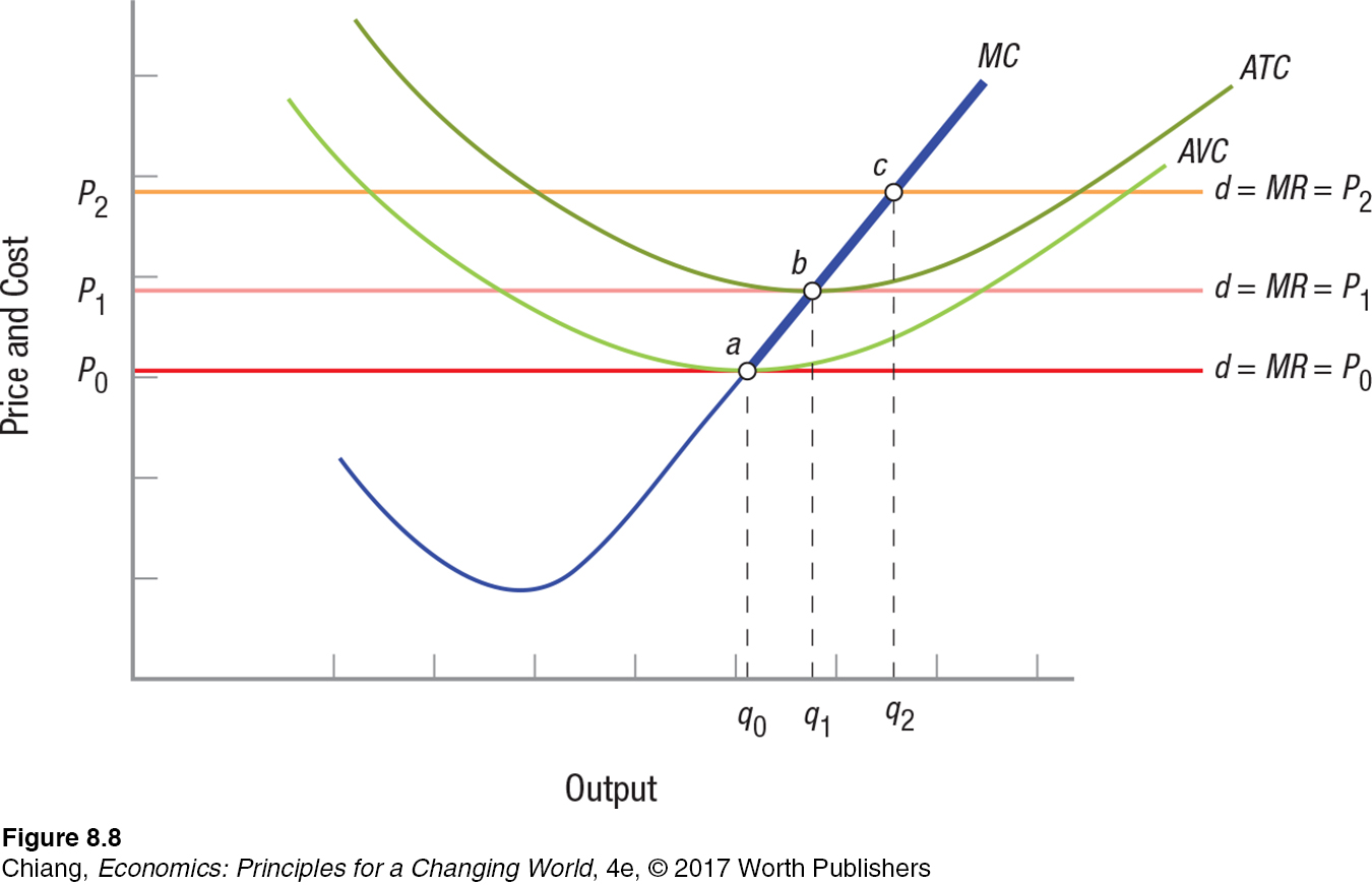
short-
From this quick summary, we can see that a firm’s short-
Keep in mind also that the short-
CHECKPOINT
PERFECT COMPETITION: SHORT-
Marginal revenue is the change in total revenue from selling an additional unit of a product.
Perfectly competitive firms are price takers, getting their price from markets, enabling them to sell all they want at the going market price. As a result, their marginal revenue is equal to product price and the demand curve facing the perfectly competitive firm is a horizontal straight line at market price.
Perfectly competitive firms maximize profit by producing that output where marginal revenue equals marginal cost (MR = MC).
When price is greater than the minimum point of the average total cost curve, firms earn economic profits.
When price is just equal to the minimum point of the average total cost curve, firms earn normal profits.
When price is below the minimum point of the average total cost curve, but above the minimum point of the average variable cost curve, the firm continues to operate, but earns an economic loss.
When price falls below the minimum point on the average variable cost curve, the firm will shut down and incur a loss equal to total fixed costs.
The short-
run supply curve of the firm is the marginal cost curve above the minimum point on the average variable cost curve.
QUESTION: Describe why profit-
Answers to the Checkpoint questions can be found at the end of this chapter.
Keep in mind that marginal cost is the additional cost to produce another unit of output, and price equals marginal revenue and is the additional revenue from selling one more unit of the product. If MR is greater than MC, the firm earns more revenue than cost by selling that next unit; therefore, the firm will sell up to the point at which MR = MC. At that last unit at which MR = MC, the firm is earning a normal profit on that unit (a positive accounting profit). When MC > MR, the firm is spending more to produce that unit than it receives in revenue and is losing money on that last unit, lowering overall profits. Thus, firms will not produce and sell all they can produce: They will produce and sell up to the point at which MR = MC.