12.3 Interpreting a Between-Subjects, Two-Way ANOVA
Interpretation of a statistical test involves stating in plain language what the results mean. The interpretation plan for a two-way ANOVA addresses the same three questions as were addressed for a one-way ANOVA but for more effects: (1) Were the null hypotheses rejected? (2) How large are the effects? (3) Where are the effects and what is their direction?
Let’s start with Dr. Ballard’s study about the impact of caffeine and sleep deprivation on mental alertness. In this study, 30 college students were randomly assigned to six groups. Before completing a mental alertness task one hour after waking up, half the participants consumed a cup of caffeinated coffee and half didn’t. Further, one third of the participants had a full night’s sleep, one third were sleep-deprived by one hour, and one third by two hours. The results of the study are shown in Figure 12.5 (see page 432) and Figure 12.7, and in Table 12.13.
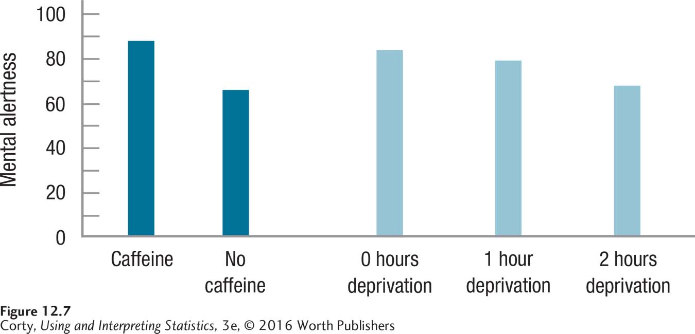
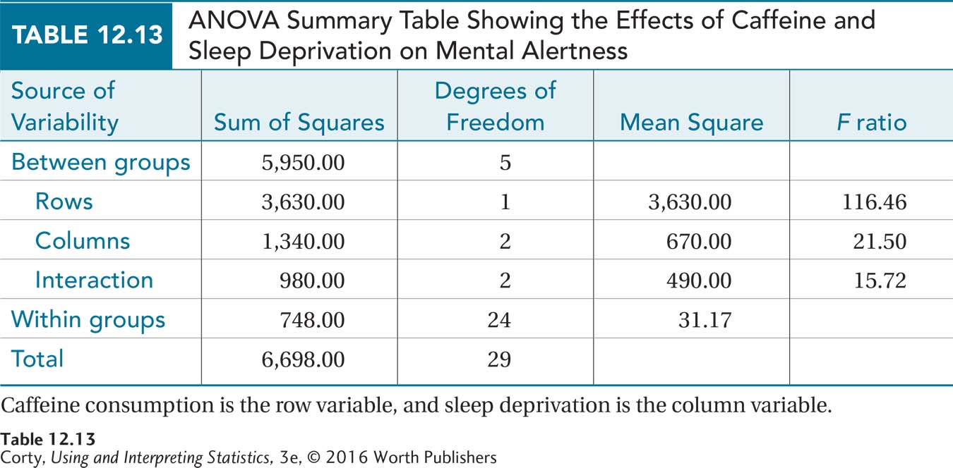
Figure 12.7 graphs the row means for the main effect of caffeine and the column means for the main effect of sleep deprivation.
Figure 12.5 uses the cell means to show what appears to be an interaction effect.
Table 12.13 shows the ANOVA summary table, from which Dr. Ballard will need a number of values as he interprets the results.
Were the Null Hypotheses Rejected?
To determine if any of the three null hypotheses was rejected—one for the row main effect, one for the column main effect, and one for the interaction effect—Dr. Ballard needs the decision rules generated in Step 4 and the F ratios calculated in Step 5. The critical values of F were Fcv Rows = 4.260, Fcv Columns = 3.403, and Fcv Interaction = 3.403. The values of F calculated were FRows = 116.46, FColumns = 21.50, and FInteraction = 15.72 (see Table 12.13). Applying the three decision rules:
116.46 ≥ 4.260, so reject H0 Rows, accept H1 Rows, and call the row effect statistically significant.
21.50 ≥ 3.403, so reject H0 Columns, accept H1 Columns, and call the column effect statistically significant.
15.72 ≥ 3.403, so reject H0 Interaction, accept H1 Interaction, and call the interaction effect statistically significant.
The next step is to write the results in APA format. APA format for the results of an ANOVA means reporting five pieces of information: (1) stating what test was done (an F test), (2) indicating the numerator and denominator degrees of freedom for the F ratio, (3) reporting the observed value of the test statistic, (4) naming the selected alpha level, and (5) telling whether the observed F fell in the rare zone (p < .05, i.e., null hypothesis was rejected) or in the common zone (p > .05, the null hypothesis was not rejected).
APA format for the main effect of rows is
F(1, 24) = 116.46, p < .05
For the main effect of columns, APA format is
F(2, 24) = 21.50, p < .05
For the interaction effect, APA format is
F(2, 24) = 15.72, p < .05
After determining the status—statistically significant or not—of each F ratio, a researcher can begin to interpret the results. It is tempting to start the interpretation with one of the main effects displayed in Figure 12.7, but remember—with a two-way ANOVA and a statistically significant interaction effect, the interaction takes precedence.
When the interaction effect is statistically significant, the null hypothesis that each main effect has an independent effect on the dependent variable is rejected. The alternative hypothesis that the two independent variables interact to affect the dependent variable in at least one cell is accepted. As a result, the main effects are less relevant. To explore further what the interaction means, Dr. Ballard will need to use a post-hoc test to compare individual cell means.
Dr. Ballard can’t be sure which mean differences are statistically significant until the post-hoc tests are completed, but inspecting Figure 12.5 gives some sense of the interaction. Figure 12.5 suggests that the amount of sleep deprivation has little effect on mental alertness when people are dosed with caffeine. However, for those who don’t receive caffeine, alertness declines as sleep deprivation increases.
What about the statistically significant main effects? Does sleep deprivation affect mental alertness? Does caffeine? Both answers are of the “it depends” variety. Look at Figure 12.5. Whether sleep deprivation affects performance depends on whether one has consumed caffeine. And, whether caffeine affects performance depends on whether a person is sleep-deprived. It doesn’t look like the main effects will add much to our interpretation.
How Big Are the Effects?
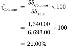
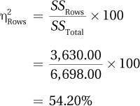
The same measure of effect, eta squared, is used for two-way ANOVA as was used for repeated-measures ANOVA. For a two-way ANOVA, eta squared can be calculated for each main effect and for the interaction. Eta squared, like r2, calculates the percentage of variability in the dependent variable that is explained by an explanatory variable or by the interaction of the explanatory variables.
The formulas for calculating eta squared for the row main effect, the column main effect, and the interaction effect are given in Equation 12.3.
Equation 12.3 Formulas for Calculating Eta Squared (η2) for Row Main Effect, Column Main Effect, and Interaction Effect
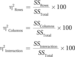
where η2Rows = eta squared for the row main effect, the percentage of variability in the dependent variable that is explained by the row explanatory variable
η2Columns = eta squared for the column main effect, the percentage of variability in the dependent variable that is explained by the column explanatory variable
η2Interaction = eta squared for the interaction effect, the percentage of variability in the dependent variable that is explained by the interaction between the row explanatory variable and the column explanatory variable
SSRows = sum of squares rows
SSColumns = sum of squares columns
SSInteraction = sum of squares interaction
SSTotal = sum of squares total
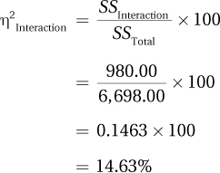
For the caffeine/sleep deprivation study, let’s start with η2 for the statistically significant interaction.
Dr. Ballard calculates eta squared for the interaction effect as follows:
The same standards are used for interpreting eta squared as were used for r2 for one-way ANOVA:
η2 ≈ 1% is a small effect.
η2 ≈ 9% is a medium effect.
η2 ≈ 25% is a large effect.
Even though the rows (caffeine) effect is very large at 54% and the column (sleep deprivation) effect at 20% is stronger than the interaction effect, the focus of the interpretation will be on the interaction. The interaction of the two variables, which explains about 15% of the variability in mental alertness, is a medium effect. Most of the variability that sleep deprivation explains is due to the effect on the no caffeine participants. The line for the caffeine-receiving participants in Figure 12.5 is mostly flat, indicating that degree of sleep deprivation explains little of the variability in mental alertness for these subjects. In contrast, the line for the no caffeine participants is on a downward trajectory as sleep deprivation increases, suggesting that amount of sleep deprivation explains a lot of the variability in mental alertness for these subjects. Does the amount of sleep deprivation explain a lot of the variability in mental alertness? It depends. The main effects are trumped by the interaction effect.
Where Are the Effects, and What Is Their Direction?
Just as with the other ANOVA tests, finding where the effects lie for two-way ANOVA involves the use of post-hoc tests. And, just as with the other ANOVAs, post-hoc tests for two-way ANOVA should be used only when the effect is statistically significant.
If the row main effect is statistically significant, and if there are three or more levels of the row explanatory variable, then a post-hoc test for the row effect can be used to find which pairs of row means differ statistically. (If there are only two row means and the row main effect is statistically significant, then the two existing row means must differ statistically.)
If the column main effect is statistically significant, and if there are three or more levels of the column explanatory variable, then a post-hoc test for the column effect can be used to find which pairs of column means differ statistically. (If there are only two column means and the column main effect is statistically significant, then the two existing column means must differ statistically.)
If the interaction effect was statistically significant, then a post-hoc test for the interaction effect can be used to find which pair(s) of cell means differ statistically.
The post-hoc test for the between-subjects, two-way ANOVA is the same one used for other ANOVAs, the Tukey HSD. HSD, remember, stands for “honestly significant difference.” If a pair of means differs by the HSD value or more than the HSD value, then the difference is a statistically significant one. The formulas for the calculation of HSD values are found in Equation 12.4.
Equation 12.4 Formulas for Calculating Tukey HSD Values for Post-Hoc Tests for Between-Subjects, Two-Way ANOVA
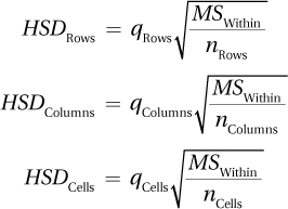
where HSDRows = HSD value for the row main effect
qRows = q value for the row main effect, from Appendix Table 5, where k = number of rows and df = dfWithin
MSWithin = within-groups mean square
nRows = number of cases in a row
HSDColumns = HSD value for the column main effect
qColumns = q value for the column main effect, from Appendix Table 5, where k = the number of columns and df = dfWithin
nColumns = number of cases in a column
HSDCells = HSD value for the interaction effect
qCells = q value for the interaction effect, from Appendix Table 5, where k = the number of cells and df = dfWithin
nCells = number of cases in a cell
For the caffeine/sleep deprivation data, there is little need to do post-hoc tests for the statistically significant main effects as our focus will be on the interaction. Instead, the HSD test will be used to interpret the interaction effect only.
The HSD to be calculated will be used to compare cell means—any two cell means that differ by the HSDCells value have a difference that is large enough to represent a statistically significant difference. And statistically significant sample differences provide evidence for population differences.
Here’s what one needs to calculate HSDCells:
Determine the alpha level, .05 or .01. Typically, the same alpha level as used in the decision rule for the F ratio is utilized. For Dr. Ballard’s study, this means α = .05.
To find the qCells value in Appendix Table 5, know that k = 6, because there are six cells, and that df = 24, because dfWithin = 24. The intersection of the column for k = 6 and the row for df = 24 gives qCells = 4.37.
From the ANOVA summary table, note that MSWithin = 31.17.
Each cell has five cases, so nCells = 5.
Here is Equation 12.4, with those values substituted:
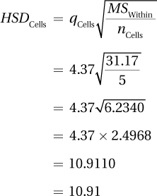
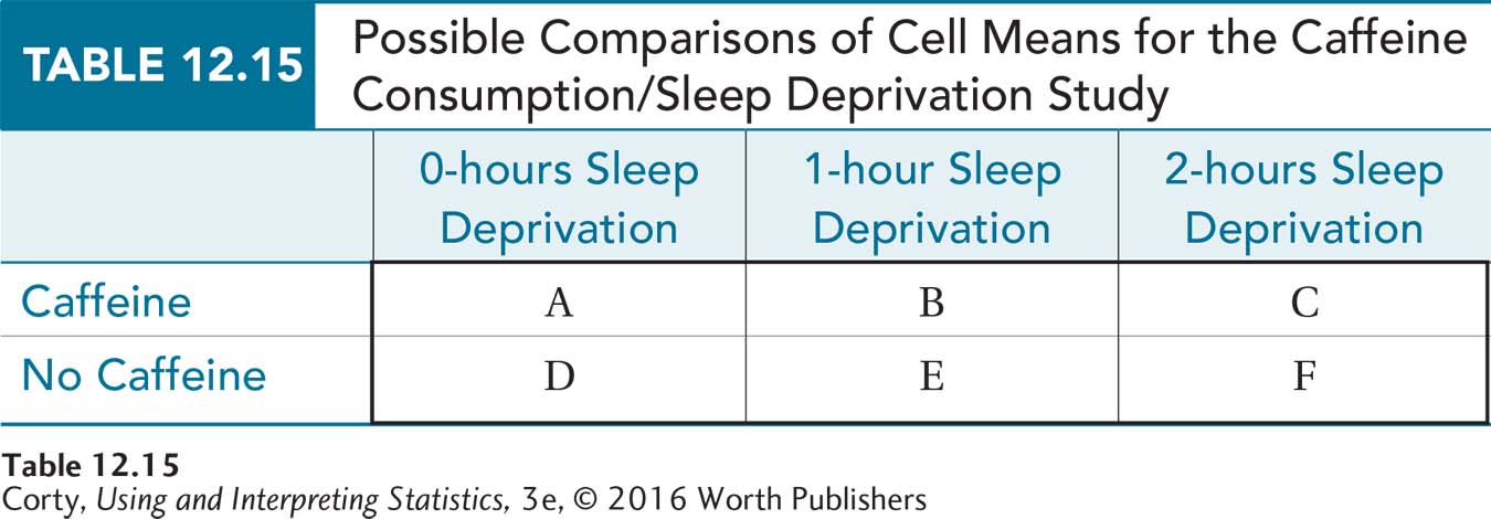
The HSDCells value is 10.91 and any two cell sample means that differ by that much or more have a statistically significant difference. Table 12.14 contains all six cell means and there are 15 possible cell-by-cell comparisons (see Table 12.15). Note, in the points below, how Dr. Ballard approaches the comparisons in an organized fashion and indicates the directions of the difference.
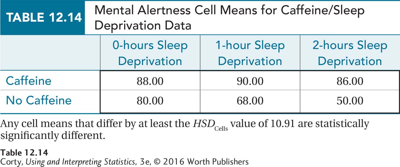
For participants who consumed no caffeine, each increase in sleep deprivation—from 0 hours (M = 80.00) to 1 hour (M = 68.00), and from 1 hour to 2 hours (M = 50.00)—caused a statistically significant decline in mental alertness.
Consuming caffeine seems to protect against the negative effects of sleep deprivation as there was no statistically significant change in cell means for the caffeine group. (The means for 0, 1, and 2 hours of sleep deprivation were, respectively, 88.00, 90.00, and 86.00.)
Looking at differences between the caffeine and no-caffeine groups, there is no evidence that caffeine consumption helped performance if no sleep deprivation occurred (means of 88.00 vs. 80.00). But, it did help performance with 1 hour of sleep deprivation (90.00 vs. 68.00) and 2 hours of sleep deprivation (86.00 vs. 50.00).
| Possible Cell-to-Cell Comparisons | |
| A vs. | B, C, D, E, and F |
| B vs. | C, D, E, and F |
| C vs. | D, E, and F |
| D vs. | E and F |
| E vs. | F |
Putting It All Together
Before writing an interpretation of a two-way ANOVA, it is helpful to review the interaction graph, Figure 12.5. The graph shows two things:
For those who don’t consume caffeine, mental alertness decreases as sleep deprivation moves from 0 hours of deprivation to 1 hour and to 2 hours.
Consuming caffeine keeps mental alertness from deteriorating, at least with 1 or 2 hours of sleep deprivation.
Here’s Dr. Ballard’s interpretation in which he addresses the following four points: What was done? What was found? What does it mean? What suggestions exist for future research?
This study explored the effects of caffeine consumption and sleep deprivation on mental alertness. Using a between-subjects design, 30 college students were assigned to six groups and then had their mental alertness tested. Half received caffeine before testing and half didn’t; one third had a full night’s sleep, one third were awakened 1 hour early, and one third 2 hours early. There was a statistically significant interaction effect of the two variables on mental alertness F(2, 24) = 15.72, p < .05 as well as statistically significant main effects for caffeine F(1, 24) = 116.46, p < .05 and sleep deprivation F(2, 24) = 21.50, p < .05. In general, caffeine consumption kept mental alertness elevated and, as sleep deprivation increased, performance deteriorated. However, these two variables did not independently affect mental alertness.
The interaction effect was moderately strong and showed that the impact of sleep deprivation on mental alertness depended on whether one consumed caffeine before testing or not. Further, how caffeine affected mental alertness depended on how sleep-deprived one was. For people who did not consume caffeine, increasing sleep deprivation caused a worsening of mental alertness. In contrast, consuming caffeine kept sleep deprivation from affecting mental alertness. This study suggests that a person can compensate for the mental alertness deficit caused by an hour or two of sleep deprivation by drinking a cup of coffee. It would be wise to replicate this study, to see if the effect is found in a different population. If it is, future research should investigate the effect of different doses of caffeine on different amounts of sleep deprivation.
(By the way, the data in this example were made up. Don’t put too much faith in caffeine being an effective antidote to sleep deprivation. Sorry.)
Worked Example 12.3
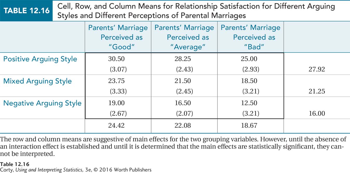
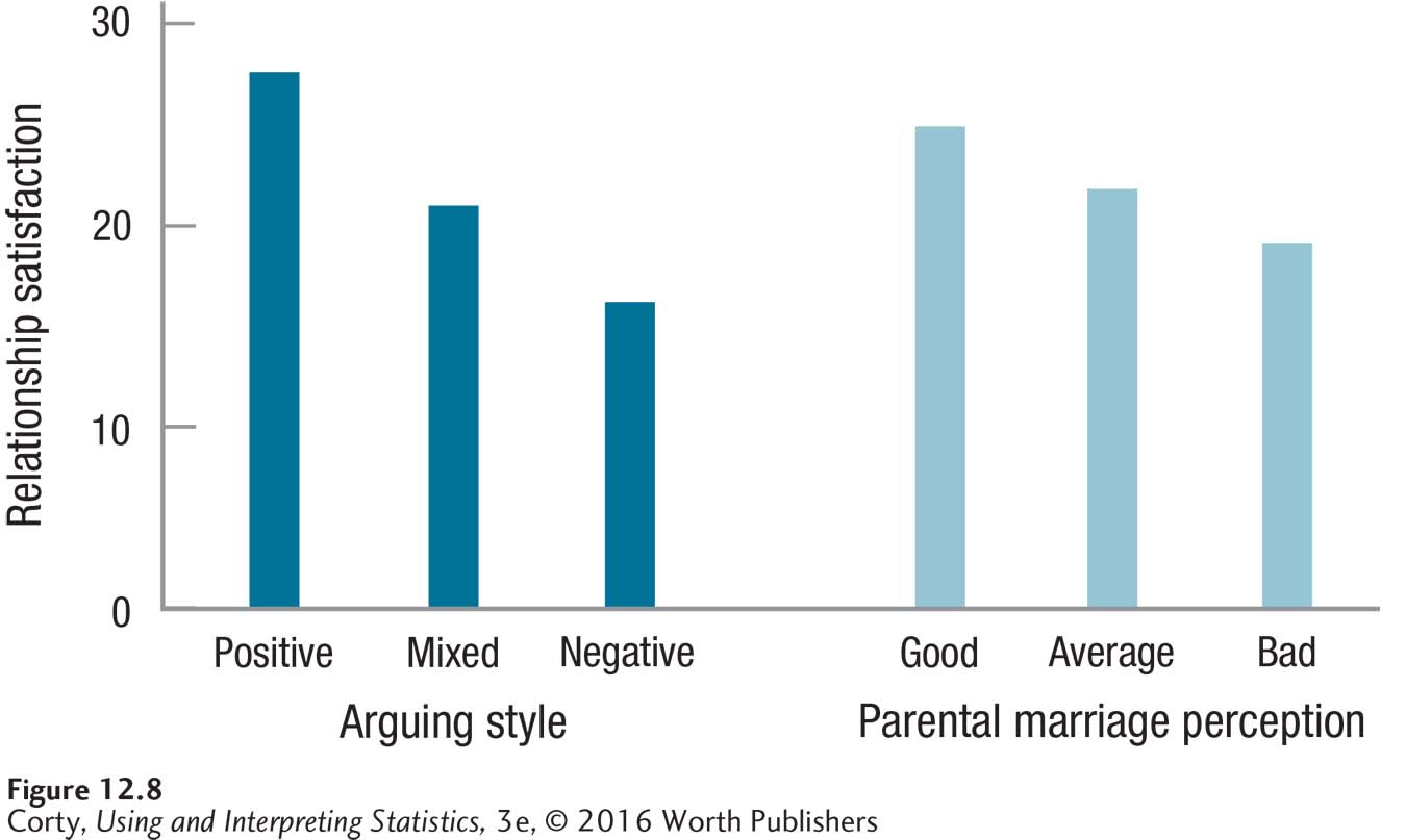
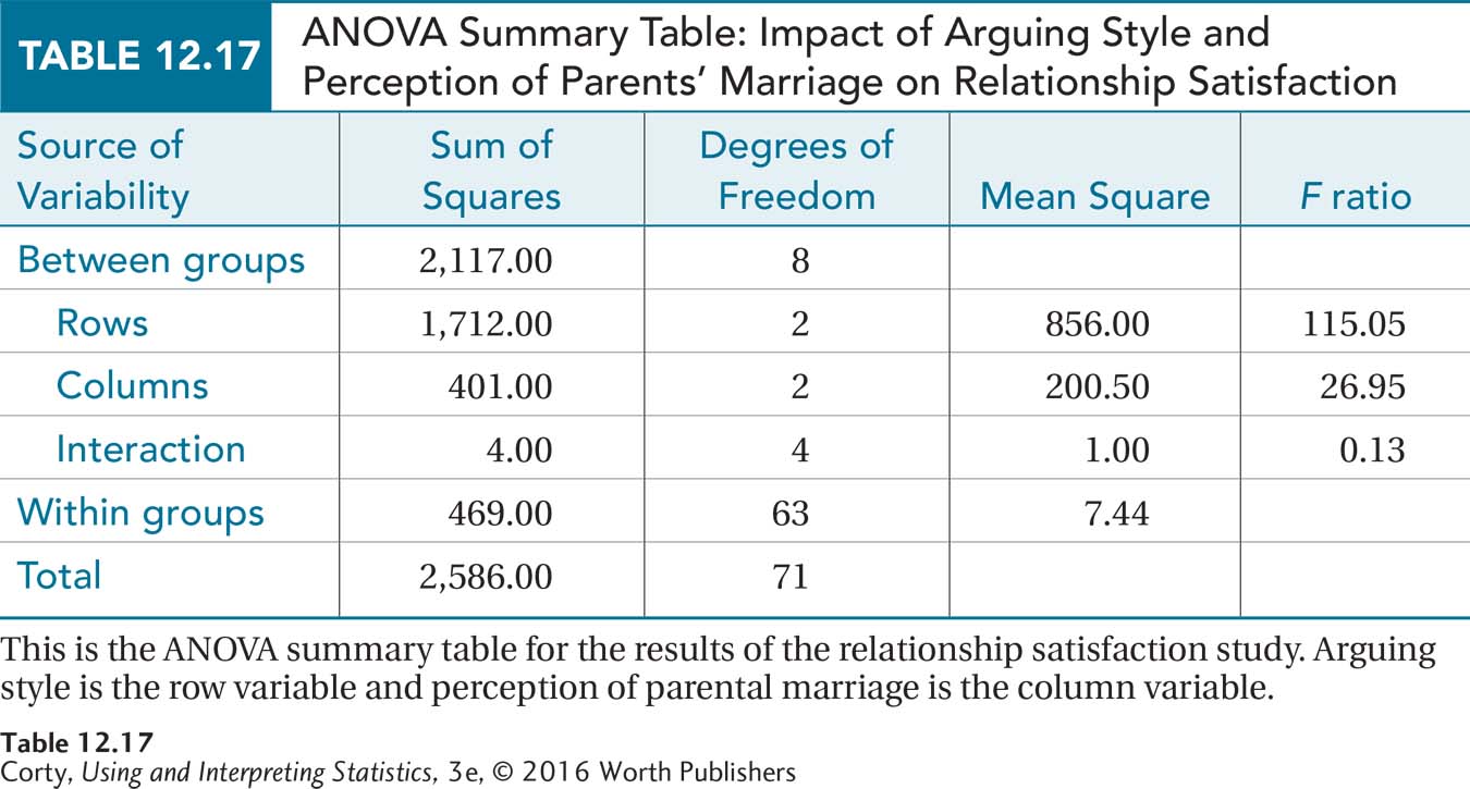
For practice in interpreting two-way ANOVA, a return to Dr. Larue’s study of factors affecting relationship satisfaction is in order. In that study, there were three levels of arguing style—positive, mixed, and negative—crossed with three different perceptions of the quality of one’s parents’ marriage—good, average, and bad. The mean level of relationship satisfaction for each of the nine conditions, measured on a scale ranging from 5 (very low) to 35 (very high), is shown in Table 12.16. The apparent lack of interaction is shown graphically in Figure 12.6. And, Figure 12.8 displays the main effects for arguing style and parental marital quality.
The three critical values of F were Fcv Rows = 3.150, Fcv Columns = 3.150, and Fcv Interaction = 2.525. The ANOVA summary table, which makes a return appearance in Table 12.17, shows that the observed values of F for the three effects were FRows = 115.05, FColumns = 26.95, and FInteraction = 0.13.
Were the null hypotheses rejected?
Row main effect: 115.05 ≥ 3.150, so reject H0 Rows and accept H1 Rows.
In APA format: F(2, 63) = 115.05, p < .05.
The row effect, arguing style, is statistically significant.
It is reasonable to conclude, in the larger population, that at least one arguing style differs from at least one other in mean relationship satisfaction.
Column main effect: 26.95 ≥ 3.150, so reject H0 Columns and accept H1 Columns.
In APA format: F(2, 63) = 26.95, p < .05.
The column effect, perception of parental marital quality, is statistically significant.
It is reasonable to conclude, in the larger population, that at least one level of perceived marital quality differs from at least one other in mean relationship satisfaction.
Interaction effect: 0.13 < 2.525, so fail to reject H0 Interaction.
In APA format: F(4, 63) = 0.13, p > .05.
The interaction effect is not statistically significant.
There is not enough evidence to conclude, in the larger population, that the effect of arguing style interacts with the effect of perceived parental marital quality to affect relationship satisfaction.
In the caffeine/sleep deprivation study, the interaction effect was statistically significant and, as a result, the statistically significant main effects were ignored. Now, in the relationship satisfaction study, the two main effects are statistically significant and the interaction is not. How does interpretation work with this set of results?
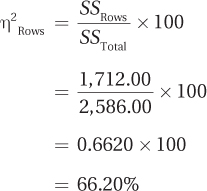
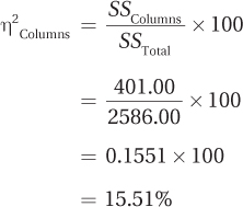
How big are the effects? Effect size is measured by calculating eta squared (Equation 12.3):
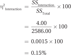
Note that eta squared for the not-statistically-significant interaction effect was calculated. Even though the interaction effect was not significant, it is possible for eta squared to be sizable. If that happened, it would serve to alert a researcher to the possibility of Type II error. In the current situation, with the percentage of variability near zero, there is nothing to make Dr. Larue think she missed finding an interaction effect that really exists. From here on out, it is safe to ignore the interaction effect.
Eta squared for the rows effect was about 66% and for the columns effect it was about 16%. Both main effects have an impact on relationship satisfaction, but one more than the other. The impact of arguing style on relationship satisfaction is quite strong. The impact of perceived parental marital quality is smaller but still meaningful. These results suggest that higher levels of relationship satisfaction are associated more with being a positive arguer than with perceiving one’s parents’ marriage as good, though having a good model of a marriage is associated meaningfully with relationship satisfaction.
Where are the effects, and what is their direction? Now it is time to use Equation 12.4 to conduct some post-hoc tests and find out what is causing the statistically significant effects. Remember, only conduct a post-hoc test when the effect is statistically significant. With the current example, Dr. Larue has no need to find out what caused the interaction effect because there is no evidence that an interaction effect exists.
To apply Equation 12.4, first find the q value from Appendix Table 5. This depends on α (.05), how many means are being compared, and what the degrees of freedom are. For both the row effect and column effect, there are three means, so k = 3 in both instances. Both instances have the same degrees of freedom as well: dfWithin = 63. Turning to Appendix Table 5, there is a column with k = 3, but no row for df = 63. In these situations, apply The Price Is Right rule and use the df value that is closest to 63 without going over. Here, that is df = 60. The q value, at the intersection of k = 3 and df = 60, is 3.40 for α = .05.
To apply Equation 12.4, one also needs to know MSWithin, which is 7.44, and how many cases are in a row and a column. Each row contains 24 cases, as does each column. All the values are the same for our calculations for HSDRows and HSDColumns: q = 3.40, MSWithin = 7.44, and n = 24, so both HSD values can be calculated in one pass:
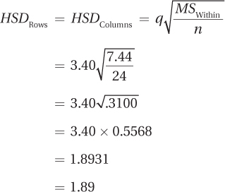
With an HSD value of 1.89, any two row means or any two column means that differ by that amount or more are statistically significantly different.
For the row main effect, relationship satisfaction grows statistically significantly worse as there is less positive arguing and more negative arguing:
Positive arguers (M = 27.92) have statistically significantly more relationship satisfaction than do mixed arguers (M = 21.25). The difference, 6.67, is greater than the HSD value of 1.89.
Mixed arguers (M = 21.25) have statistically significantly more relationship satisfaction than do negative arguers (M = 16.00). The difference, 5.25. is greater than the HSD value.
For the column main effect, relationship satisfaction gets statistically significantly worse as the perception of the parents’ marriage worsens:
Students who rated their parents’ marriage as good (M = 24.42) rated their own relationship as statistically significantly more satisfying than those who rated their parents’ marriage as average (M = 22.08). The difference, 2.34, is greater than the HSD value of 1.89.
Rating one’s parents’ marriage as average (M = 22.08) is associated with a statistically significantly higher score on relationship satisfaction than rating it as bad (M = 18.67). The difference, 3.41, is greater than the HSD value.
Page 457Putting it all together. Before writing her four-point interpretation, Dr. Larue reviewed the graph displaying the main effects (Figure 12.8), so she had a clear picture of the results in her mind. Here’s what she wrote (notice, this is a quasi-experimental study in which nothing is manipulated, so she avoids cause-and-effect language to describe the results):
In this social psychology study, the abilities of two variables, arguing style and perceived quality of parental marriage, to predict relationship satisfaction in college students were examined. Students were classified into three categories of arguing style (positive, negative, or mixed) and with three different perceptions of their parents’ marriages (good, average, or bad). Eight students from each of these possible combinations who were in current relationships were randomly selected and completed a survey measuring degree of satisfaction with their current relationship.
Using a between-subjects, two-way ANOVA, both arguing style and parental marital perception had statistically significant effects on relationship satisfaction [respectively, F(2, 63) = 115.05, p < .05, and F(2, 63) = 26.95, p < .05]. There was no interaction effect for the two variables F(4, 63) = 0.13, p > .05.
Arguing style was the stronger predictor of relationship satisfaction. As students’ arguing style moved from positive to negative, there was a decrease in relationship satisfaction. The role played by perceived parental marriage, though less powerful, was still meaningful. A more negative view of parents’ marriages was associated with lower relationship satisfaction.
This study suggests that the relationships one sees as a child influence one’s future relationship satisfaction. The good news is that a more powerful influence on relationship satisfaction is arguing style and a positive arguing style is a skill that can be learned. Future research should examine whether teaching positive arguing skills improves relationship satisfaction.
Practice Problems 12.3
12.08 Given α = .05, dfRows = 3, dfColumns = 2, dfInteraction = 6, dfWithin = 60, FRows = 3.25, FColumns = 1.22, and FInteraction = 0.83, (a) write each result for this between-subjects, two-way ANOVA in APA format and (b) for each result report whether the effect is statistically significant.
12.09 Given this ANOVA summary table, (a) calculate η2 for each effect and (b) classify each effect as small, medium, or large. Use α = .05.
| Source of Variability | Sum of Squares | Degrees of Freedom | Mean Square | F ratio |
| Between groups | 5,357.00 | 15 | ||
| Rows | 3,725.00 | 3 | 1,241.67 | 37.63 |
| Columns | 1,312.00 | 3 | 437.33 | 13.25 |
| Interaction | 320.00 | 9 | 35.56 | 1.08 |
| Within groups | 7,392.00 | 224 | 33.00 | |
| Total | 12,749.00 | 239 |
12.10 Here is a table of cell means for a 3 × 2 between-subjects, two-way ANOVA with seven cases in each cell. Note that the row means and column means have been calculated.
| Column 1 | Column 2 | Column 3 | ||
| Row 1 | 26.00 | 30.00 | 34.00 | 30.00 |
| Row 2 | 18.00 | 22.00 | 26.00 | 22.00 |
| 22.00 | 26.00 | 30.00 |
Here is the between-subjects, two-way ANOVA summary table for these data:
| Source of Variability | Sum of Squares | Degrees of Freedom |
Mean Square | F ratio |
| Between groups | 1,120.00 | 5 | 224.00 | |
| Rows | 672.00 | 1 | 672.00 | 35.99 |
| Columns | 448.00 | 2 | 224.00 | 12.00 |
| Interaction | 0.00 | 2 | 0.00 | 0.00 |
| Within groups | 672.00 | 36 | 18.67 | |
| Total | 1,792.00 | 41 |
As appropriate, calculate HSD values and comment on the direction of the differences for the effects.
12.11 A kinesiologist wanted to investigate the effect of temperature and humidity on human performance. He found 28 college students and randomly assigned them to four different conditions, during which they were to walk at their normal pace on a treadmill for 60 minutes. He measured how far, in miles, they walked. The conditions varied in temperature and humidity: (1) normal temperature and normal humidity; (2) normal temperature and high humidity; (3) high temperature and normal humidity; (4) high temperature and high humidity. The results looked like this:
| Normal Humidity | High Humidity | ||
| Normal Temperature | 3.00 miles | 2.80 miles | 2.90 |
| High Temperature | 2.80 miles | 2.00 miles | 2.40 |
| 2.90 | 2.40 |
Here is the ANOVA summary table:
| Source of Variability | Sum of Squares | Degrees of Freedom |
Mean Square | F ratio |
| Between groups | 4.13 | 3 | ||
| Rows | 1.75 | 1 | 1.75 | 25.00 |
| Columns | 1.75 | 1 | 1.75 | 25.00 |
| Interaction | 0.63 | 1 | 0.63 | 9.00 |
| Within groups | 1.58 | 24 | 0.07 | |
| Total | 5.71 | 27 |
The critical value of F for each effect is 4.260. Eta squared for the row, column, and interaction effects, respectively, are 30.65%, 30.65%, and 11.03%. The HSD value for comparing cells is 0.39. Given all this information, write a four-point interpretation.
Application Demonstration
The two examples offered in this chapter so far—Dr. Ballard’s caffeine/sleep deprivation study and Dr. Larue’s relationship satisfaction study—have both involved statistically significant results. Unfortunately, research doesn’t always turn out that way. Here’s an example of a two-way ANOVA study in which not one of the three null hypotheses is rejected. How are results interpreted in this situation?
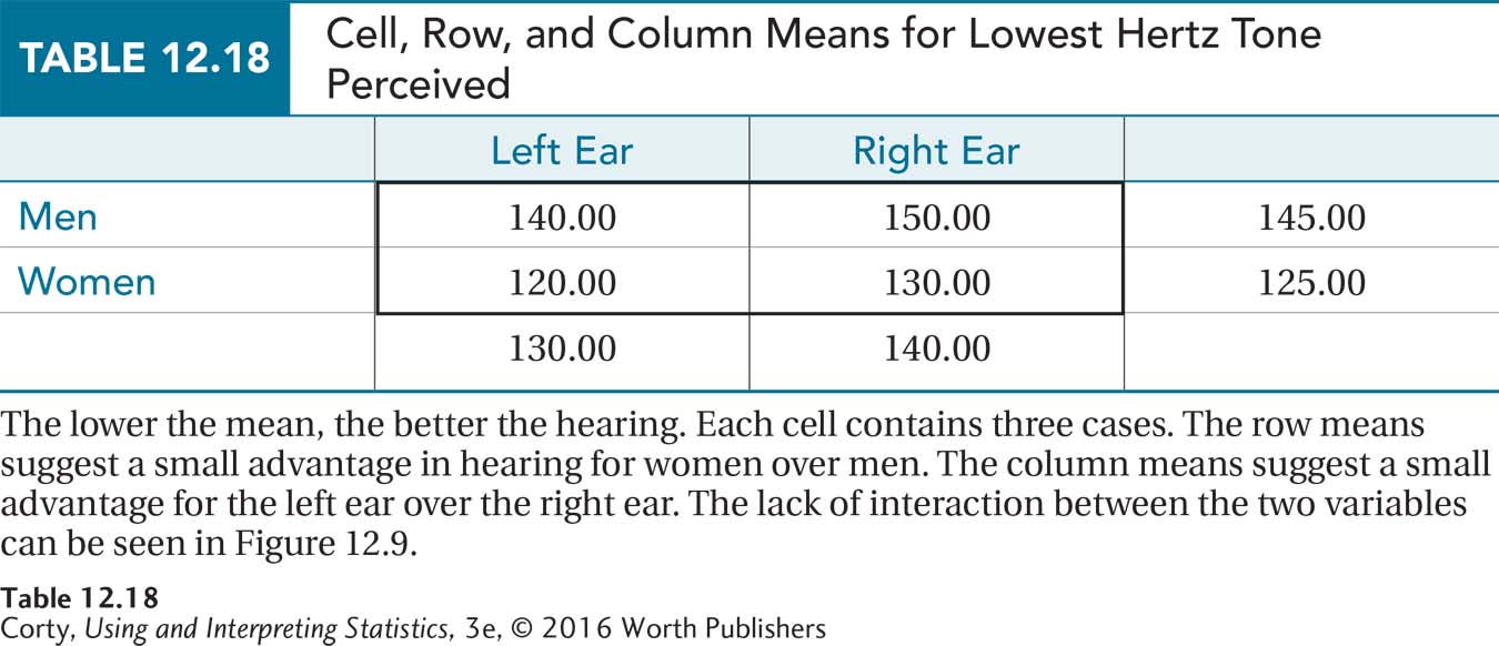
Imagine a sensory psychologist, Dr. Porter, who wanted to explore the threshold for perceiving low-frequency sounds. She tested six men and six women to see how low a sound they could perceive. Half the participants were tested in their left ears and half in their right ears. Sounds were measured in hertz (Hz), and the lower the hertz the better a person’s hearing. (Want to see how well you do? Search for “Ultimate Sound Test [10000 Hz–1 Hz]” on YouTube.)
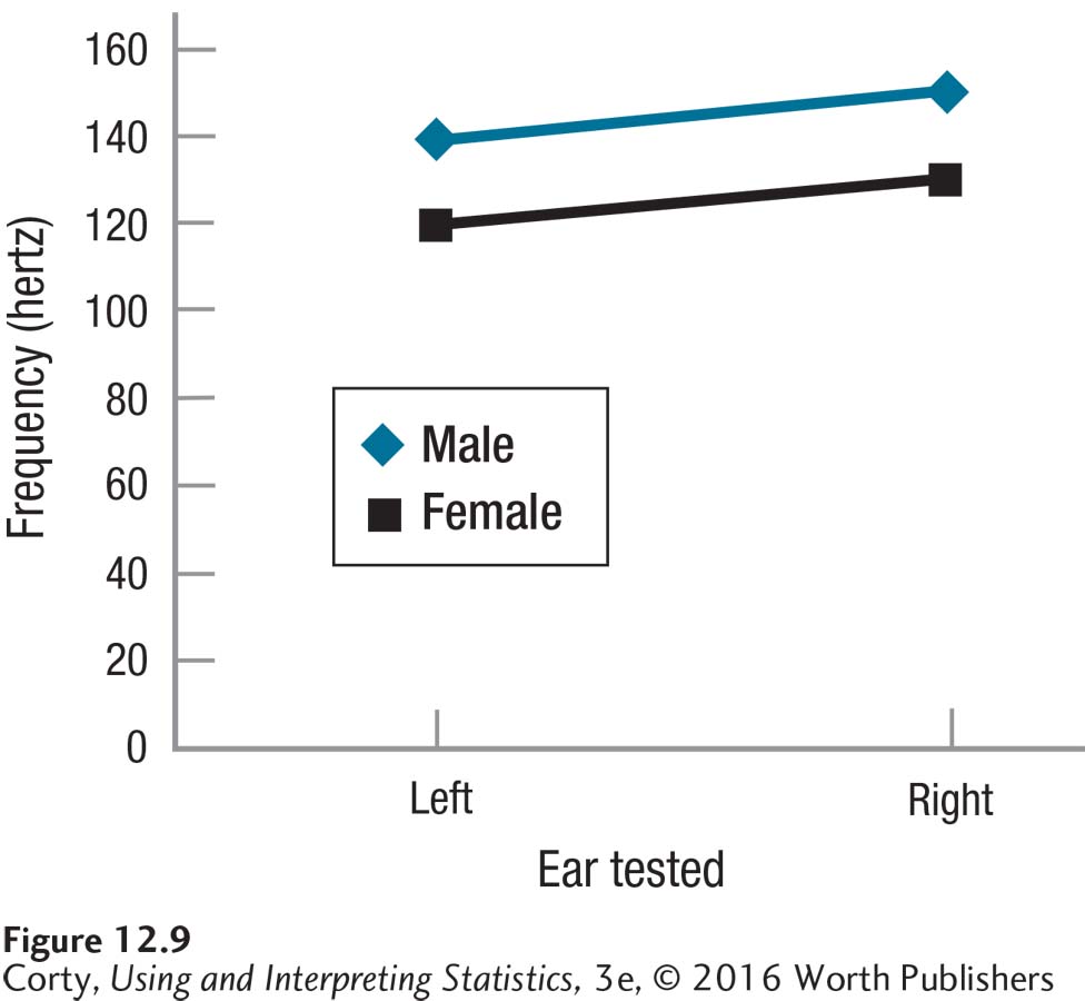
Table 12.18 and Figure 12.9 show the results. There appears to be no interaction and slightly better performance exists (a) for women and (b) for the left ear. Whether the effects are statistically significant or can be explained by sampling error remains to be seen.
The appropriate statistical test to compare the four means from these two independent variables is a two-way ANOVA. The four groups are all independent samples, so the test is a between-subjects, two-way ANOVA, specifically a 2 × 2 ANOVA.
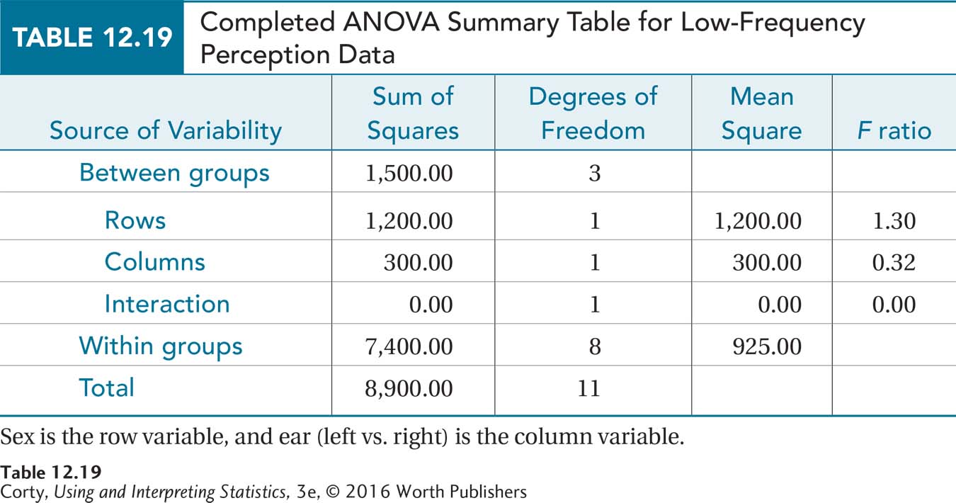
No assumptions were violated and the ANOVA summary table is presented in Table 12.19. The critical value of F for all three effects was 5.318 and no effect was statistically significant.
There is not enough evidence to conclude that men and women differ in their ability to hear low-frequency sounds.
There is not enough evidence to conclude that the right ear differs from the left ear in its ability to hear low-frequency sounds.
There is not enough evidence to conclude that a person’s sex and which ear is tested interact to influence the perception of low-frequency sounds.
With no statistically significant effect, no need exists to do any post-hoc testing. A researcher would be wise, however, to calculate eta squared in order to consider the possibility of a Type II error, the possibility of having failed to find an effect that does occur.
Applying Equation 12.3, Dr. Porter finds
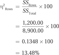
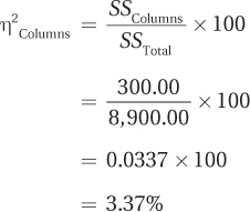
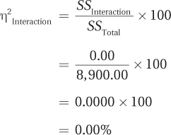
These results show that the row main effect, η2 = 13.48%, is medium. The column main effect, η2 = 3.37%, is small. There is no interaction effect. Not enough evidence exists to say that the row effect of sex—male vs. female—affects the perception of low frequencies, but there is enough of a hint here that Dr. Porter might want to draw attention to it. As always, looking at a picture of the effects, like that shown in Figure 12.9, helps to clarify what the effects were. Here’s her four-point interpretation:
A sensory psychologist conducted a study testing the ears (left vs. right) of both men and women to see if one ear or one sex had a lower threshold for low-frequency sounds. According to this study, there was not enough evidence to conclude that either one sex or one ear was better than the other at perceiving low-frequency sounds. However, the results suggested that women (M = 125.00 Hz) may have an edge over men (M = 145.00 Hz) in perceiving low-frequency sounds. To investigate this, it would be advisable to replicate the study with a larger sample size.