13.4 Calculating a Partial Correlation
We started this chapter with a scatterplot showing that there was an association between the number of community hospitals per state and the number of deaths per state. That correlation did not mean that having hospitals caused the deaths. Rather, it seemed more plausible that a confounding variable, the population of a state, caused both the number of hospitals and the number of deaths. Now, we are going to learn about a technique called partial correlation that can be used to quantify objectively if and how a confounding variable exerts influence.
A confounding variable is a third variable, let’s call it Z, that is not measured and/or not controlled, that correlates with both X and Y, and that potentially explains why X and Y are correlated. Here is an example. Suppose we give $10 each to ten 21-year-old college students on a Friday night and ask them to rendezvous with us at midnight. When they return, we find out how much money they spent and measure how well they can walk a straight line. We find a relationship—the more money a student has spent, the worse he or she is at walking the line. Clearly, a third variable, the amount of alcohol a student has purchased, would explain both why his or her funds are depleted and why his or her performance is impaired. If we took into account each student’s alcohol consumption, the correlation between money spent and performance would be explained.
A partial correlation mathematically removes the influence of a third variable on a correlation. It is a useful technique that moves a correlational study a little bit in the direction of an experimental study. Partial correlations do not allow cause-and-effect conclusions to be drawn, but they can make potential cause-and-effect conclusions less or more plausible. In the student study above, if the results turned out as described, it would be less plausible to conclude that spending money is the cause of impaired performance.
How can a partial correlation make a cause-and-effect conclusion more plausible? Suppose a researcher finds a relationship between the number of years a person has smoked cigarettes and the degree of impairment of lung function. This researcher claims that the impairment is caused by smoking. Another researcher points out that people who have been smoking longer are usually older, and posits that it is age that causes the impaired lung function. If the effect of age is removed and the correlation between years of smoking and impaired lung function remains strong, then the notion that it is the number of years of smoking that leads to impaired lung function remains plausible.
The abbreviation for a partial correlation is rXY–Z, the correlation between X and Y minus the influence of Z. The formula for a partial correlation, shown in Equation 13.6, makes use of three pieces of information: the correlation between X and Y, the correlation between X and Z, and the correlation between Z and Y.
Equation 13.6 Partial Correlation of X with Y, Controlling for Z
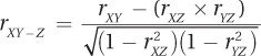
where rXY–Z = the partial correlation of X and Y controlling for the influence of Z
rXY = the correlation between X and Y
rXZ = the correlation between X and Z
rYZ = the correlation between Y and Z
Let’s use a partial correlation to control for the effect of population on the correlation between the number of community hospitals per state and the number of deaths per state. The scatterplot in Figure 13.1 at the start of this chapter shows a strong and direct relationship. Not surprisingly, the correlation is strong and significant: r(23) = .89, p < .05. But, the correlation between the number of hospitals (X) and the state population (Z) was .92, and for the number of deaths (Y) and the population, it was .98.
Using rXY = .89, rXZ = .92, and rYZ = .98, we can complete Equation 13.6:
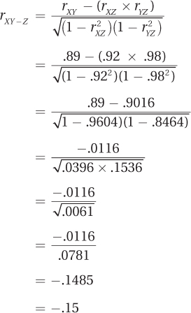
The correlation of the number of hospitals with the number of deaths was .89. But, when population was controlled for, the correlation fell to –.15. It went from statistically significant to failing to reject the null hypothesis. This means that there is not enough evidence to suggest the number of community hospitals has any causal impact on the number of deaths in a given state—the apparent association between the two variables can be explained by the states’ populations.
A Common Question
Q How many degrees of freedom does a partial correlation have?
A df for a partial correlation is N – 3. For the community hospital study, there were 25 states, so df = 25 – 3 = 22. The critical value of r is ± .396; thus, the observed r of –.15 falls in the common zone. The results would be reported as r(22) =–.15, p > .05.
Worked Example 13.3
A researcher gathered a random sample of 160 students at her college and measured their physical and mental health on two dimensions: the distance that they are able to run in 30 minutes and happiness, as indicated on a survey. She theorized, from a biopsychosocial perspective, that if there is a mind–body connection, then a relationship should exist between physical health and psychological health. She found in her sample that the correlation between the two variables was .37 [r(158) = .37, p < .05], suggesting that a correlation does indeed exist between physical health and mental health.
She tells a colleague, an obesity researcher, about these findings, and the colleague suggests that the observed relationship could be explained by the body mass index (BMI)—people with high BMIs are in poorer mental and physical health. Luckily, the biopsychosocial researcher had recorded the heights and weights of her subjects, so she calculates BMIs and finds that the correlation between physical health and BMI is .42; for BMI and emotional health, it is .18. Using these values, she calculates a partial correlation:
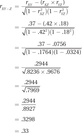
The partial correlation of .33 is reduced slightly from .37, but it is still statistically significant: r(157) = .33, p < .05. The relationship between physical and emotional health is not explained by BMI.
Practice Problems 13.4
13.21 Using N = 54, rXY = .53, rXZ = .46, and rYZ = .25, calculate rXY–Z.
13.22 Using N = 27, rXY = .35, rXZ = .18, and rYZ = .17, calculate rXY–Z.
Application Demonstration
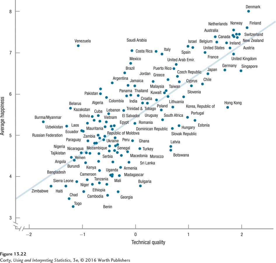
To see how the Pearson r is used in real research, let’s examine a study that involves both psychology and political science. A researcher wanted to know if living in a nation with better government services was associated with greater happiness. He used the average happiness ratings reported by citizens of 130 nations (Ott, 2011). Happiness ratings by individuals could range from 0 (“Right now I am living the worst possible life”) to 10 (“Right now I am living the best possible life”). The individual ratings were averaged together to yield a score for a country. The country with the greatest average happiness was Denmark (M = 8.00) and the lowest average happiness was Togo (M = 3.24); the United States was near the top (M = 7.26).
The researcher also developed a measure of government services for each of the 130 nations. Nations that provided better public services had better regulations, experienced less corruption, etc., received higher scores on government services.
The scatterplot showing the relationship between the two variables can be seen in Figure 13.22. The r value for these data is .75, and the results are statistically significant [r(128) = .75, p < .05]. There is a positive relationship between the two variables in these countries—better government services are associated with happier citizens. Squaring the correlation gives the effect size, r2 = 56.25%. According to Cohen (1988), this is a large effect.
The 95% confidence interval for ρ ranges from .66 to .82. Note that (1) the confidence interval doesn’t capture zero, (2) the bottom end (.66) is far from zero, and (3) the confidence interval is quite narrow. One can conclude that there is probably a strong, positive correlation between these two variables in the larger population of countries.
The researcher thought of government services as predicting, or leading to, happiness. But, do better government services cause more happiness? This is a correlational study where nothing is manipulated. All that one can be sure of is that there is an association between better government services (X) and more happiness (Y). Correlation is not causation, so we shouldn’t draw conclusions about cause and effect.
When two variables are correlated, three possible explanations exist for the correlation:
Y causes Y.
Y causes X.
Some other variable, Z, causes X and Y.
For the happiness/government services data, all three explanations are plausible. First, it is possible that X causes Y, that better government services lead to more happiness. This seems sensible—if government provides better services to its citizens, then their lives should be better and they should be happier.
The second explanation, Y causes X, also seems plausible. Happier citizens could cause better government. It seems possible that happier people will make their government function better because they are more likely to vote, more willing to serve on committees, less likely to disobey laws, and so on.
The third explanation—that Z causes both X and Y—is plausible if one can think of a third variable, Z, that has an impact on both X and Y. Wealth is a third variable that springs to mind. Nations with more wealth might have better government services because they can afford to spend more money on providing them. And, nations with more wealth might have happier citizens because, well, because money does help buy happiness. So, perhaps wealth causes both better government services and more happiness.
Untangling cause and effect in a correlational study is a challenge for any researcher. Looking at the scatterplot (Figure 13.22) and the .75 r value, there is clearly an association between the two variables. Just as clearly, the relationship is a direct one. But, how can a researcher put the results in context and explain what they mean? Here’s an interpretation that addresses, even embraces, the uncertainty.
A researcher examined the relationship between the quality of government services and happiness in 130 nations around the world. He found that there was a strong, positive association between these two variables [r(128) = .75, p <.05]. This means that governments with better services had happier citizens. One explanation for the observed relationship is that countries with better government services provide an environment that leads to more happiness among their citizens. Improving government then should raise up citizens.
But, this study is correlational and other explanations are possible. Perhaps the relationship goes in the other direction. That is, happy citizens lead to better government because happy citizens are more likely to be involved civically and to be concerned for, and supportive of, the welfare of others.
There is a third explanation for the correlation between these two variables, an explanation that also seems plausible. Another variable may exist, called a confounding variable, that causes both good government and citizen happiness. Examples of potential confounding variables are how wealthy a nation is and how industrialized it is. Nations with more wealth, for example, can afford to provide more government services. And, for individual people, maybe money does buy some happiness. Thus, it seems reasonable to suggest replicating this study with confounding variables being measured so their influence can be assessed.