15.5 Other Nonparametric Tests
In this brief section, two other nonparametric tests are introduced: the Spearman rank-order correlation coefficient and the Mann–Whitney U.
The Spearman Rank-Order Correlation Coefficient
The Spearman rank-order correlation coefficient (abbreviated Spearman r or rs) is the nonparametric version of the Pearson correlation coefficient. The Spearman r examines the relationship between (1) two ordinal-level variables, (2) one ordinal-level variable and one interval/ratio-level variable, or (3) as a fallback option with two interval/ratio-level variables when the assumptions for the Pearson r have been violated.
One can think of the Spearman r as a Pearson r in which the correlation is calculated for data that are converted to ranks. This means that a researcher can directly apply the hypothesis-testing steps about hypotheses, decision rules, calculation, and interpretation from the Pearson r to the Spearman r—as long as he or she remembers that ordinal, or ranked, data are being used.
For an example of how the Spearman r works, imagine a psychologist who examined the relationship between romantic attractiveness and academic success in high school students. His measure of romantic attractiveness was an interval scale that ranged from 0 (low) to 10 (high). Class rank, an ordinal measure, was the measure of academic success. He obtained both of these measures on a random sample of 24 seniors, and Panel A in Figure 15.6 shows the relationship between them. It appears as if students who are doing less well academically are more romantically attractive.
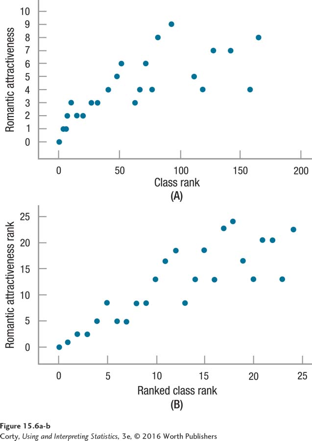
Class rank is an ordinal-level variable, so a Pearson r is not appropriate to use to analyze these data. Instead, a Spearman r is the appropriate test. To conduct the Spearman r, each variable is assigned a rank from 1 to 24 and the rankings are correlated. Why is each variable assigned a rank from 1 to 24? Because there are 24 cases in the sample. The scatterplot for the ranked data is displayed in Panel B of Figure 15.6, and it shows a very similar pattern to Panel A.
Look at class rank on the X-axis in the top panel of Figure 15.6. For these 24 students, it ranges from 1 to 165 and the X-axis goes all the way up to 200 to accommodate this. Then look at the X-axis in the bottom panel—instead of ranging from 0 to 180, it ranges from 0 to 25. That’s because the Spearman r takes class rank, which was already an ordinal-level variable, and turns it into pure ranks. The student with the worst class rank in this sample, who had a class rank of 165, now has a score of 24, which indicates the worst class rank in the sample.
Similarly, the Y-axis variable, romantic attractiveness, is converted into ranks. In Panel A, the scores ranged from 0 to 10. In Panel B, when the scores are ranked, the highest possible score (for the most attractive person) is now 24, not 10.
The Spearman r is just like the Pearson r, except that it correlates ranks, not raw scores. The difference between the two can be seen in the axes of the two scatterplots in Figure 15.6. In addition, look closely at the shape of the two scatterplots in Figure 15.6—they are similar, but not exactly the same. Converting raw scores to ranks can change the shape. Sometimes, as here, it makes the relationship appear stronger. Other times it makes the relationship appear weaker. However, making the relationship stronger or weaker isn’t the objective. The objective is to use the appropriate statistical test for the data. If correlating two ordinal variables, one ordinal variable with one interval or ratio variable, or two interval and/or ratio variables where it’s not possible to proceed with a Pearson r, then the Spearman rank-order correlation coefficient is the appropriate test.
The Mann–Whitney U Test
The Mann–Whitney U test is the nonparametric equivalent of the independent-samples t test. It is used to compare two independent populations when the dependent variable is measured at the ordinal level, or as a fallback test when nonrobust assumptions for an independent-samples t test have been violated. Because it uses an ordinal outcome variable, the Mann–Whitney U test determines if the median of one population is significantly different from the other.
The Mann–Whitney U works by combining the two independent samples and then assigning a rank to each case based on its standing in the pooled group. The two samples are then separated, and the sum of the ranks for each of the samples is calculated and used to calculate U. If the two populations have similar scores on the dependent variable, then each sample will have a mixture of high ranks and low ranks. However, if the two populations differ, then one will have more high ranks than the other. When this happens, the U value will reflect the difference in ranks between the samples, and the null hypothesis of no difference in the medians will be rejected.
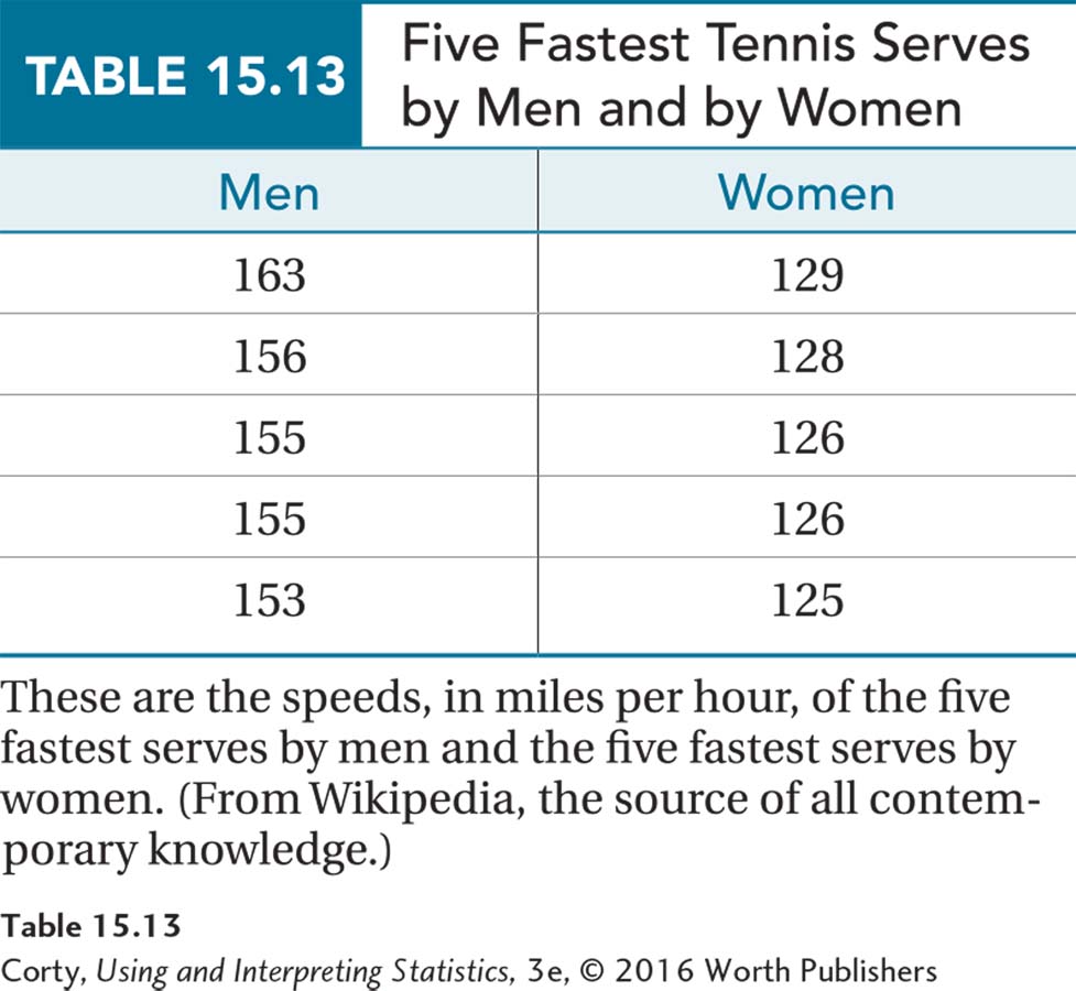
Here’s an example where the difference between the two samples is very obvious. Table 15.13 shows the speeds, in miles per hour, of the five fastest tennis serves by men and the five fastest serves by women. Clearly, the fastest male tennis serves are faster than the fastest female tennis serves. Let’s see how the Mann–Whitney U test would show this.
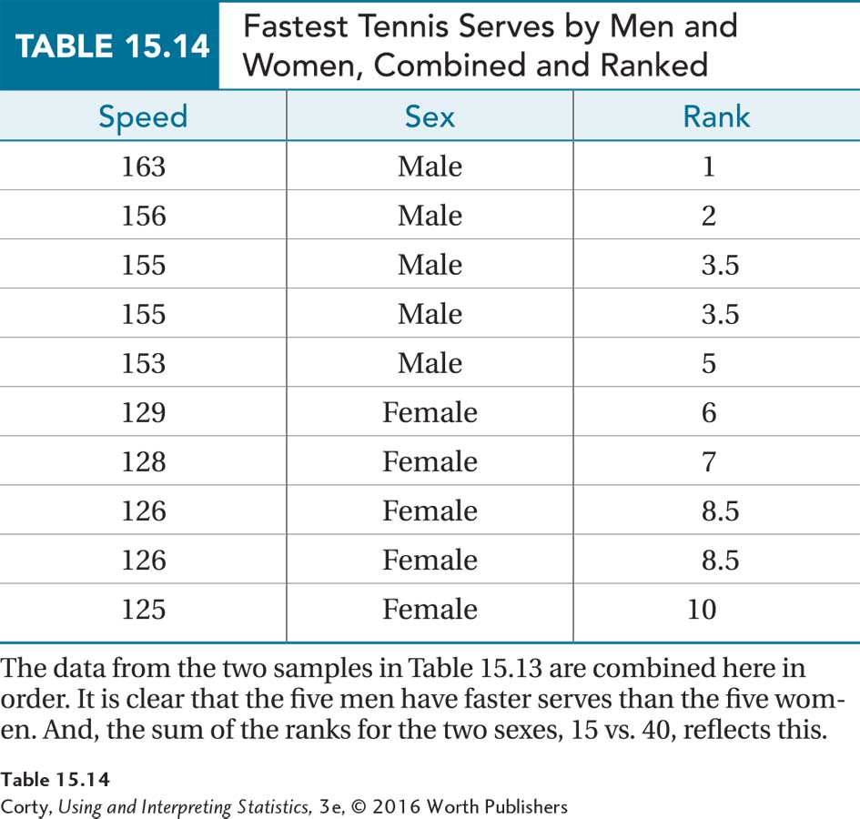
In Table 15.14, the two samples are combined into one group and the cases are ordered from fastest to slowest. The rank of 1 is given to the fastest serve and the rank of 10 to the slowest serve. There is no overlap in the ranks assigned to men and women. Ranks 1 to 5 belong to the men and ranks 6 through 10 to the women. The sum of the men’s ranks, 15, and the sum of the women’s ranks, 40, are very different numbers. And, the U value that the Mann–Whitney U test would calculate for these data would reflect as much.
That’s how the Mann–Whitney U test works. It combines the two samples into one group, assigns ranks to the whole group, then puts the cases back into their original samples, and compares the ranks. If the ranks are evenly distributed between the two samples, then there is no evidence that the populations differ. But if one sample has a lot of high ranks and the other a lot of low ranks, then the difference between the populations is statistically significant.
Practice Problems 15.4
For these practice questions, select the appropriate statistical test from the following: Pearson r, Spearman r, independent-samples t test, or Mann–Whitney U test.
15.13 A psychologist wanted to examine the relationship, in adolescents, between days of drug use in the past year and IQ score. Days of drug use turned out to be very positively skewed.
15.14 The psychologist then divided the adolescents into two groups, those with no days of drug use over the past year and those with one or more days. She wanted to compare the two groups in terms of IQ.
15.15 A sports economist wanted to know if countries that invested more in their sports programs did better in the Olympics. He divided countries into those that competed in 10 or more sports in the summer Olympics and those that competed in fewer than 10 sports. For each country, he found its medal count rank, and he divided this by the number of sports in which the country competed to obtain his dependent variable, rank per events entered.
Application Demonstration
To see chi-square in action, let’s analyze some data from a real-life study. A group of researchers was interested in determining if survival after surgery was influenced by a person’s nutritional status before surgery. They took almost 400 patients about to undergo surgery for kidney cancer and classified them as malnourished or not. Surgery was then performed and the researchers followed the patients for three years to see how many lived and how many died (Morgan et al., 2011).
Step 1 Pick a Test. Though the researchers used more complex statistical techniques, we’ll apply a chi-square test of independence to the data:
The grouping variable, nutritional status, is nominal with two categories: (1) malnourished or (2) not malnourished.
The dependent variable, survival three years later, is nominal with two categories: (1) alive or (2) dead.
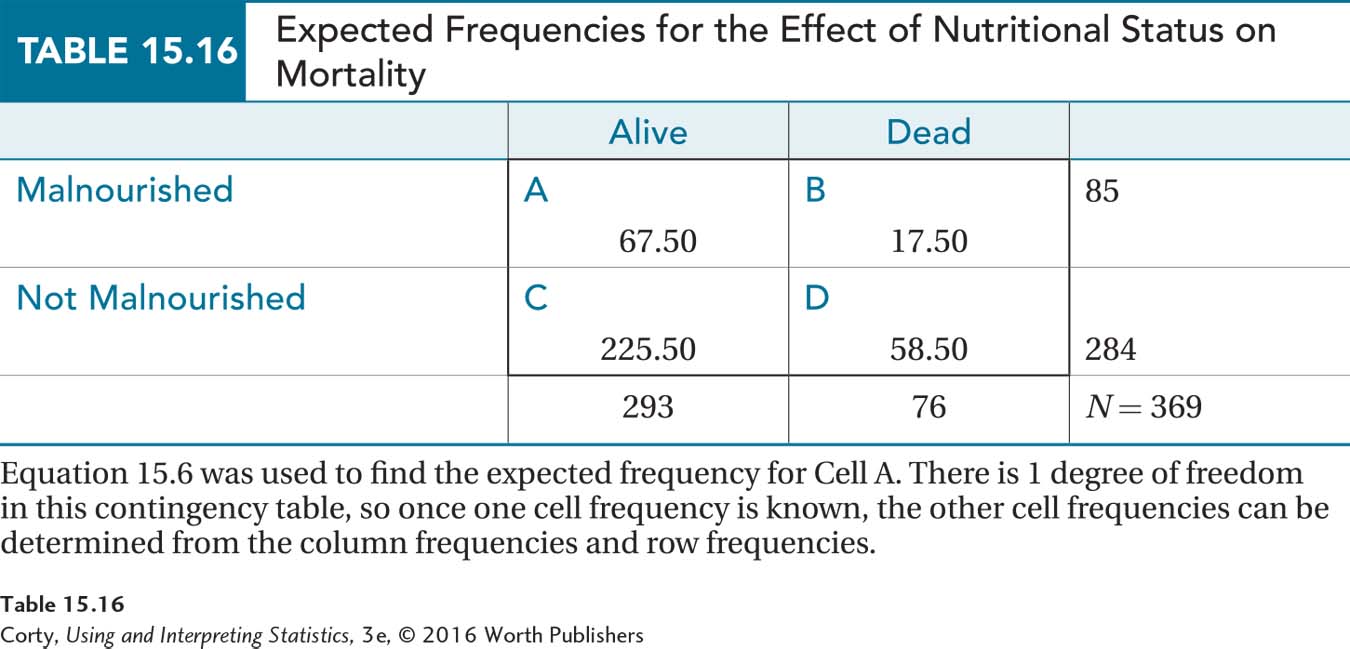
Table 15.15 displays the results as a contingency table. The table shows cell frequencies, as well as row percentages and column percentages. Eighty-five of the 369 patients (23%) were classified as malnourished and 76 of the 369 patients (21%) died within three years.
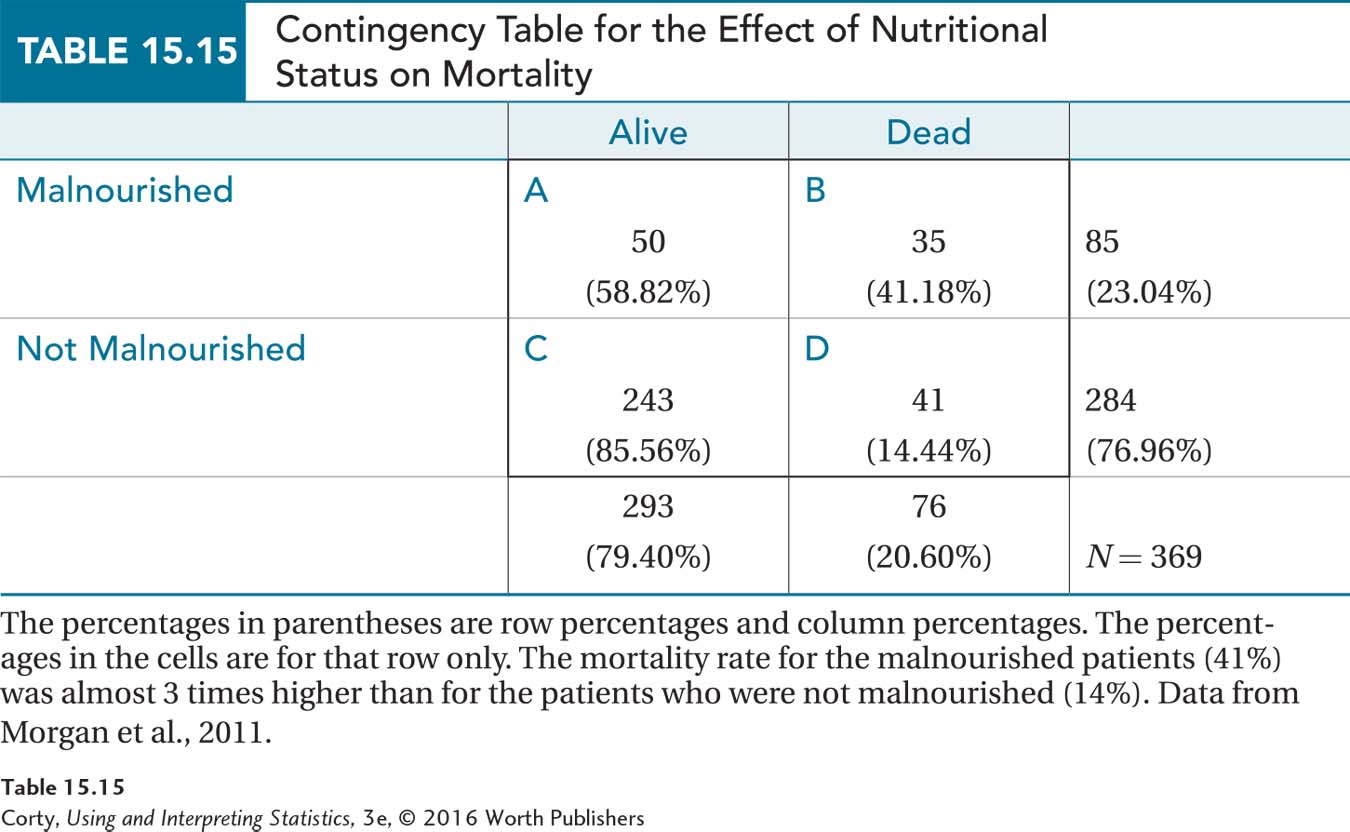
The percentages in the cells suggest that being malnourished prior to surgery diminishes one’s chance of surviving for three years after surgery: 35 of the 85 malnourished patients died—that’s 41%—compared to only 41 of the 284 not malnourished patients, or 14%. In other words, there appears to be a relationship between malnourishment status and mortality status. But, is this a statistically significant relationship? To answer that question about these nominal-level variables, a chi-square test of independence is required.
Step 2 Check the Assumptions.
Random samples. The sample was not a random sample, leaving uncertainty about the population to which the results can be generalized. The sample is large; it might be representative of patients with kidney cancer at this hospital. Whether these patients are like patients at other hospitals or in other states and countries is unknown. The random samples assumption is robust to violation, so it’s OK to proceed with the planned chi-square test of independence.
Page 602Independence of observations. No evidence exists that the patients influenced each other. There’s no reason to believe any patients were in the study twice. The independence of observations assumption does not appear to have been violated.
Adequate expected frequencies. All cells must have expected frequencies of at least 5. This assumption can’t be assessed until the expected frequencies are calculated.
Step 3 List the Hypotheses. The null hypothesis says that malnutrition status and survival are independent and the alternative hypothesis states that they have some relationship:
H0: ρ = 0
H1: ρ ≠ 0
Step 4 Set the Decision Rule. The alpha level is set at .05, as usual. The degrees of freedom are calculated using Equation 15.4:
df = (R – 1) × (C – 1)
= (2 – 1) × (2 – 1)
= 1 × 1
= 1
Use Appendix Table 9 to find the critical value of chi-square, χ2cv = 3.841. Here is the decision rule:
If χ2 ≥ 3.841, reject H0 and say the results are statistically significant.
If χ2 < 3.841, fail to reject H0 and say the results are not statistically significant.
Step 5 Calculate the Test Statistic. To save time, the expected frequencies for the cells are shown in Table 15.16. Equation 15.5 was used to calculate the expected frequency for Cell A and then logic was utilized to find the expected frequencies for the other three cells. None of the expected frequencies is less than 5, so it’s now known that the third assumption was not violated.
Using Equation 15.3, the chi-square value is calculated as 28.63:
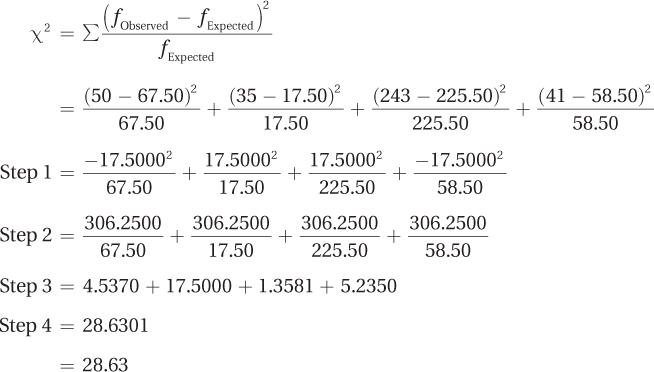
Step 6 Interpret the Results. The calculated value of chi-square (28.63) is greater than the critical value (3.841), so the null hypothesis is rejected and the results are written in APA format as χ2(1, N = 369) = 28.63, p < .05. A statistically significant difference exists between the mortality rate for malnourished patients and patients who were not malnourished. There are only two groups, so we know the direction of the difference: the mortality rate is higher for malnourished patients than for patients who were not malnourished, 41% vs. 14%.
Using Equation 15.7, Cramer’s V is calculated as .28:
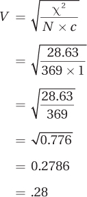
By Cohen’s standards (1988), this is a medium effect. However, Cohen’s standards are meant as guidelines. A change in the mortality rate from 14% to 41%—almost a threefold increase—seems like a strong effect, especially as death is the outcome.
Putting it all together.
Data were analyzed from a study in which researchers compared the mortality rate for kidney cancer patients who were and were not malnourished prior to surgery. Three years after surgery, 41% of the malnourished patients had died compared to only 14% of the patients who were not malnourished. This almost threefold increase in mortality was a statistically significant difference [χ2(1, N = 369) = 28.63, p < .05]. The effect seems to be a strong one. For kidney cancer patients undergoing surgery, being malnourished prior to surgery is associated with almost a threefold increase in the risk of dying in the next three years. In future studies, it would be important to assess the reason for the malnourishment. If it resulted from having a more aggressive form of cancer, it might be the cancer, not the malnourishment, that led to the increase in mortality.
DIY
What can grocery shopping tell us about gender equality? Do men do more shopping than women? Are women more likely than men to be accompanied by children?
Make a data collection sheet like the one below. Then go to a grocery store during the day and put a tally mark in Cell A for every woman you see shopping with children. A mark goes in Cell B for every woman shopping by herself. Similarly, use Cell C to keep track of men shopping with children and D for men shopping alone.
Add together Cells A and B, and Cells C and D. Use a chi-square goodness-of-fit test with expected percentages of 50% and 50% to see if men and women share shopping responsibility equally. Do the results say something about contemporary gender roles?
| Shopping with Children |
Shopping without Children |
|
| Female Shoppers |
A | B |
| Male Shoppers |
C | D |
Next, let’s see if one sex is more likely to shop with children. To do so, use the values in all four cells as the observed frequencies for a chi-square test of independence.