CHAPTER EXERCISES
Answers to the odd-numbered exercises appear in Appendix B.
Review Your Knowledge
15.01 The statistical tests in previous chapters all had ____-level or ____-level outcome variables.
15.02 ____ tests are for nominal-level or ____-level outcome variables.
15.03 The independent-samples t test is an example of a ____ test.
15.04 Parametric tests assume that the outcome variable is ____ in the population.
15.05 If a researcher violates a nonrobust assumption for a parametric test, then a nonparametric test can be used as a ____ test.
15.06 Nonparametric tests are less restricted by ____ than are ____ tests.
15.07 Nonparametric tests usually have less ____ than ____ tests.
15.08 The chi-square goodness-of-fit test is a ____-sample test used with a ____ outcome variable.
15.09 The chi-square goodness-of-fit test sees if the difference between what is ____ and what is ____ can be explained by sampling error.
15.10 The abbreviation for chi-square is ____, where the Greek letter is pronounced ____.
15.11 The sample in a chi-square goodness-of-fit test should be a ____ from the population.
15.12 There should be at least ____ cases in each cell in a chi-square goodness-of-fit test.
15.13 The chi-square goodness-of-fit test compares the distribution of the outcome variable in the ____ to the specified distribution in the ____.
15.14 The critical value of chi-square is abbreviated ____.
15.15 If the ____ lands in the ____ of the sampling distribution of chi-square, then the null hypothesis is rejected.
15.16 The degrees of freedom for a chi-square goodness-of-fit test depend on the number of ____ in the study.
15.17 If the differences between the observed frequencies and the expected frequencies in a chi-square goodness-of-fit test are small, the null hypothesis is ____.
15.18 It is impossible / possible for expected frequencies in a chi-square goodness-of-fit test to be fractional numbers.
15.19 The expected frequencies in a chi-square goodness-of-fit test add up to ____.
15.20 The first step in calculating a chi-square is to ____ the expected frequencies from the ____.
15.21 In APA format for a chi-square goodness-of-fit test, the first number inside the parentheses represents the ____.
15.22 In APA format, if the results are written “p > .05,” this means the results fell in the ____ zone.
15.23 The direction of the results for a chi-square goodness-of-fit test needs to be determined if the results are ____.
15.24 The chi-square test of independence differs from the chi-square goodness-of-fit test in terms of the number of ____ in the test.
15.25 The chi-square test of independence can be conceptualized as a ____ test or a ____ test.
15.26 To conduct a chi-square test of independence, construct a ____ table that cross-tabulates the values of the ____ with the levels of the ____.
15.27 In a contingency table, each ____ is placed in one, and only one, ____.
15.28 The assumptions for the chi-square test of independence are the same as for the ____.
15.29 The null hypothesis for the chi-square test of independence states that the ____ and the ____ are ____.
15.30 The hypotheses for a chi-square test of independence are stated the same way as they are for a ____.
15.31 The degrees of freedom for a chi-square test of independence depend on the number of ____ and the number of ____.
15.32 The formula for the chi-square test of independence is similar to / not similar to the formula for the chi-square goodness-of-fit test.
15.33 The number of cases in the rows in a chi-square test of independence add up to ____%.
15.34 The sum of the expected frequencies for the rows in a chi-square test of independence are the same as the sum of the observed frequencies for the ____.
15.35 In a Spearman rank-order correlation coefficient, the ____ of the two variables are correlated.
15.36 The ____ is the nonparametric alternative to the independent-samples t test.
15.37 The Mann–Whitney U test takes two independent ____, combines them into one ____, and then assigns a ____ to each case in the combined group.
15.38 The Mann–Whitney U test compares the ranks of the cases in one ____ to the ____ of the cases in the other sample.
Apply Your Knowledge
Pick the correct test from the following: the chi-square goodness-of-fit test, chi-square test of independence, Spearman rank-order correlation coefficient, and Mann–Whitney U test.
15.39 A high school principal developed a theory that caffeinated sodas cause more burping than decaffeinated sodas. She obtained a large sample of students and randomly assigned them to drink sodas with or without caffeine. She then waited 15 minutes and classified each student as having burped or not having burped during that time. What test should she use?
15.40 The principal also kept track of how many burps each student produced. For both the caffeinated and de-caffeinated groups, the number of burps was extremely positively skewed. What statistical test should she use to see if the number of burps differs between the two groups?
15.41 A social psychologist assigned ranks to all the second-grade boys in a school based on how much the other boys liked them. He then did the same thing for all the boys again, but based the ranks on how much the girls liked them. What test should the psychologist conduct to see if there’s an association between how boys and how girls view boys?
15.42 A statistics teacher looked out at her class of 32 students and noted that 21 of them were female. Assuming there are equal numbers of males and females in the world, what test should this teacher use to see if her class is overpopulated with women?
Checking the assumptions for a chi-square goodness-of-fit test or a chi-square test of independence
15.43 A sociologist planned to study patterns of criminality in small towns. She drew a random sample of 50 small towns from all across America. Before conducting her study, she wanted to make sure that her sample was representative of small towns. From the FBI, she learned that 2% of small towns have experienced a murder over the past 10 years. Can she use a chi-square goodness-of-fit test to compare the percentage of small towns that had experienced a murder to the national percentage?
15.44 An addictions researcher wants to see if male and female alcoholics differ in the type of alcohol they consume. She goes to a large alcohol detox facility, gets a sample of men and a sample of women, and checks each person’s chart to find the beverage of choice. She classifies the beverages as (a) wine, (b) beer, or (c) hard liquor. The table that follows shows the expected frequencies. Can the researcher use a chi-square test of independence to analyze her data?
| Beer | Wine | Hard Liquor | |
| Men | 9.07 | 8.53 | 6.40 |
| Women | 7.93 | 7.47 | 5.60 |
Stating the hypotheses for chi-square tests
15.45 State the null and alternative hypotheses for Exercise 15.43.
15.46 State the null and alternative hypotheses for Exercise 15.44.
Finding degrees of freedom for chi-square goodness-of-fit tests
15.47 Given this matrix, how many degrees of freedom are there for this chi-square goodness-of-fit test?
15.48 Given this matrix, how many degrees of freedom are there for this chi-square goodness-of-fit test?
15.49 Given this matrix, how many degrees of freedom are there for this chi-square test of independence?
15.50 Given this matrix, how many degrees of freedom are there for this chi-square test of independence?
Finding χ2cv and setting the decision rule. Use α = .05.
15.51 (a) If df = 2, what is χ2cv? (b) What is the decision rule?
15.52 (a) If df = 4, what is χ2cv? (b) What is the decision rule?
Calculating expected frequencies for a chi-square goodness-of-fit test
15.53 Given N = 97 and the expected percentages below, find the expected frequencies:
| A 63% | B 37% |
15.54 Given N = 182 and the expected percentages below, find the expected frequencies:
| A 14% | B 38% | C 48% |
Calculating χ2 for a chi-square goodness-of-fit test
15.55 Given the information in the following matrix, calculate χ2:
| fObserved | 9 | 14 | 18 | ∑ = 41 |
| fExpected | 6.97 | 15.58 | 18.45 | ∑ = 41.00 |
15.56 Given the information in the following matrix, calculate χ2:
| fObserved | 28 | 23 | 20 | ∑ = 71 |
| fExpected | 33.37 | 19.98 | 17.65 | ∑ = 71.00 |
15.57 Given the information in the following matrix, calculate χ2:
| fObserved | 40 | 50 |
| f% Expected | 35% | 65% |
15.58 Given the information in the following matrix, calculate χ2:
| fObserved | 22 | 37 |
| f% Expected | 42% | 58% |
Using APA format with α = .05
15.59 If df = 1, N = 43, χ2 = 4.81, and χ2cv = 3.841, write the results in APA format.
15.60 If df = 3, N = 78, χ2 = 5.99, and χ2cv = 7.815, write the results in APA format.
15.61 If df = 4, N = 55, and χ2 = 9.49, write the results in APA format.
15.62 If df = 5, N = 234, and χ2 = 3.85, write the results in APA format.
Determining the direction of the difference for a statistically significant chi-square goodness-of-fit test
15.63 Given the information below, determine the direction of the results:
| Category I | Category II | |
| fObserved | 24 | 26 |
| fExpected | 8.77 | 41.23 |
15.64 Given the information below, determine the direction of the results:
| Category I | Category II | |
| fObserved | 37 | 23 |
| fExpected | 49.23 | 10.77 |
Interpreting chi-square goodness-of-fit test
15.65 Dr. Lowry investigated whether fortunetellers have extrasensory perception. He obtained a random sample of 124 fortunetellers. For each one, a card was randomly selected from a well-shuffled 52-card deck and placed face down. Then the fortuneteller had to determine if the card was red or black. For each fortuneteller, Dr. Lowry recorded if he or she guessed correctly. If that person had no ESP ability, then he or she had a 50% chance of guessing correctly. Dr. Lowry found that 72 of the 124 fortunetellers (58.06%) correctly guessed the color of the card and 52 (41.94%) were wrong. The table below shows the observed and expected frequencies. The chi-square goodness-of-fit test results were χ2(1, N = 124) = 3.23, p > .05. Write a four-point interpretation.
| Guessed Correctly | Category Incorrectly | |
| fObserved | 72 | 52 |
| fExpected | 62.00 | 62.00 |
15.66 According to the U.S. government, 68% of American adults weigh more than they should. A dietician, Dr. Christiansen, maintained a theory that drinking 8 or more glasses of water a day was associated with not being overweight. She obtained a random sample of 580 American adults who consumed 8 or more glasses of water a day, weighed each adult, and classified each one as overweight or not. The table below shows the observed frequencies and the expected frequencies. The chi-square goodness-of-fit test results were χ2(1, N = 580) = 15.62, p < .05. Write a four-point interpretation.
| Not Overweight | Overweight | |
| fObserved | 230 | 350 |
| fExpected | 185.60 | 394.40 |
Completing all six steps of hypothesis testing for a chi-square goodness-of-fit test
15.67 A consumer psychologist, Dr. Wessells, obtained a random sample of 880 people who had strong preferences as to what cola they preferred. He gave each one, individually, a taste test in which each participant tasted four different colas and then had to pick his or her favorite. Dr. Wessells wondered whether consumers would be able to tell the difference. If they couldn’t, they would have a 25% chance of being right and a 75% chance of being wrong. It turned out that 279 participants correctly chose their preferred cola and 601 chose incorrectly. Use hypothesis testing to decide if all colas taste the same, even to people who have strong preferences.
15.68 Dr. Constantinople, a cancer physician, wondered whether wearing a hat protected one against skin cancer. From prior research, she knew that about 1% of adults develop skin cancer every year. She obtained a random sample of 2,040 adults who wore hats and followed them for a year. During that year, 14 developed skin cancer and 2,026 did not. Use hypothesis testing to determine if wearing a hat is associated with a change in the risk of developing skin cancer.
Generating contingency tables
15.69 A researcher compared people in their 20s, 40s, and 60s in terms of whether they supported gay marriage or not. Support was measured as a “yes” or “no.” Create a labeled contingency table that could be used to cross-tabulate the results.
15.70 An experimental group and a control group were compared in terms of whether they recovered from an illness in 5 or fewer days, 6 to 10 days, or more than 10 days. Make a labeled contingency table that could be used to cross-tabulate the results.
Finding the number of cases per row and column for a chi-square test of independence
15.71 Given the contingency table below, find the number of cases for each row and column:
| Outcome A | Outcome B | |
| Group I | 34 | 86 |
| Group II | 67 | 113 |
15.72 Given the contingency table below, find the number of cases for each row and column:
| Outcome A | Outcome B | |
| Group I | 28 | 12 |
| Group II | 32 | 18 |
Calculating expected frequencies
15.73 Given N = 72 and the information in the following contingency table, calculate the expected frequencies for the cells:
| Outcome 1 | Outcome 2 | ||
| Group I | A | B | 34 |
| Group II | C | D | 38 |
| 30 | 42 |
15.74 Given N = 123 and the information in the following contingency table, calculate the expected frequencies for the cells:
| Outcome 1 | Outcome 2 | ||
| Group I | A | B | 34 |
| Group II | C | D | 32 |
| Group III | E | F | 57 |
| 27 | 96 |
Calculating χ2
15.75 Given the information below, calculate χ2:
| Observed Frequencies | ||
| Outcome A | Outcome B | |
| Group I | 28 | 12 |
| Group II | 12 | 12 |
| Expected Frequencies | ||
| Outcome A | Outcome B | |
| Group I | 25.00 | 15.00 |
| Group II | 15.00 | 9.00 |
15.76 Given the information below, calculate χ2:
| Observed Frequencies | ||
| Outcome A | Outcome B | |
| Group I | 35 | 55 |
| Group II | 67 | 40 |
| Expected Frequencies | ||
| Outcome A | Outcome B | |
| Group I | 46.60 | 43.40 |
| Group II | 55.40 | 51.60 |
15.77 Given the information below, calculate χ2:
| Observed Frequencies | ||
| Outcome A | Outcome B | |
| Group I | 14 | 21 |
| Group II | 18 | 18 |
15.78 Given the information below, calculate χ2:
| Observed Frequencies | ||
| Outcome A | Outcome B | |
| Group I | 6 | 18 |
| Group II | 30 | 10 |
Types of error
15.79 Given χ2(1, N = 45) = 4.92, p < .05, which type of error does the researcher need to worry about?
15.80 Given χ2(1, N = 88) = 3.45, p > .05, which type of error does the researcher need to worry about?
Determining the direction of the difference
15.81 The chi-square yielded statistically significant results. Given the information below, determine the direction of the difference:
| Observed Frequencies | ||
| Outcome A | Outcome B | |
| Group I | 6 | 18 |
| Group II | 30 | 10 |
| Expected Frequencies | ||
| Outcome A | Outcome B | |
| Group I | 13.50 | 10.50 |
| Group II | 22.50 | 17.50 |
15.82 The chi-square yielded statistically significant results. Given the information below, determine the direction of the difference:
| Observed Frequencies | ||
| Outcome A | Outcome B | |
| Group I | 12 | 19 |
| Group II | 17 | 9 |
| Expected Frequencies | ||
| Outcome A | Outcome B | |
| Group I | 15.77 | 15.23 |
| Group II | 13.23 | 12.77 |
Calculating and interpreting Cramer’s V
15.83 Given χ2(3, N = 78) = 8.92, p < .05 where R = 4 and C = 2, (a) calculate V; (b) classify the effect as small, medium, or large; and (c) determine if the researcher should worry about Type II error.
15.84 Given χ2(1, N = 102) = 3.53, p > .05 where R = 1 and C = 1, (a) calculate V; (b) classify the effect as small, medium, or large; and (c) determine if the researcher should worry about Type II error.
Interpreting a chi-square test of independence
15.85 Tennis players are more likely to win points when they are serving. A tennis journalist wondered whether the server’s advantage diminished as a rally lasted longer. She randomly selected 209 points from all the matches played at the major tennis tournaments during a year. For each point, she recorded whether the rally was short (the ball went back and forth no more than twice before the point was decided) or the rally was long (the ball went back and forth more than two times). She also recorded whether the server won the point or not. The table below shows the results. She found χ2(1, N = 209) = 3.93, p < .05 and calculated Cramer’s V = .14. Write a four-point interpretation.
| Observed Frequencies | ||
| Server Wins | Server Loses | |
| Short rally | 66 | 41 |
| Long rally | 49 | 53 |
| Expected Frequencies | ||
| Server Wins | Server Loses | |
| Short rally | 58.88 | 48.12 |
| Long rally | 56.12 | 45.88 |
15.86 A college dean noticed that political science seemed to attract more male majors than psychology. She wondered if her observation were true. So, she obtained a random sample from each major and recorded the sex of each student. The table below shows her results. The dean found χ2(1, N = 55) = 3.66, p > .05; V = .26. Write a four-point interpretation.
| Observed Frequencies | ||
| Female | Male | |
| Psychology | 23 | 13 |
| Political science | 7 | 12 |
| Expected Frequencies | ||
| Female | Male | |
| Psychology | 19.64 | 16.36 |
| Political science | 10.36 | 8.64 |
Completing all six steps of hypothesis testing
15.87 A surgeon decided to compare sutures and staples in closing incisions. When he finished operating on a patient, he flipped a coin in order to determine if he would use sutures or staples to close the wound. Six months later, he called each patient and found out whether he or she was satisfied, yes vs. no, with how the scar looked. The results appear below. Use hypothesis testing to determine if there’s a difference in satisfaction between the two techniques.
| Observed Frequencies | ||
| Not Satisfied | Satisfied | |
| Sutures | 8 | 13 |
| Staples | 9 | 12 |
15.88 A political scientist developed a theory that after an election, supporters of the losing candidate removed the bumper stickers from their cars faster than did supporters of the winning candidate. The day before a presidential election, he randomly selected parking lots, and at each selected parking lot, he randomly selected one car with a bumper sticker and recorded which candidate it supported. The day after the election, he followed the same procedure with a new sample of randomly selected parking lots. For both days, he then classified the bumper stickers as supporting the winning or losing candidate. Below are the results. Use hypothesis testing to see if a difference exists between how winners and losers behave.
| Observed Frequencies | ||
| Winner | Loser | |
| Before | 34 | 32 |
| After | 28 | 10 |
Expand Your Knowledge
15.89 Complete the following contingency table. If it can’t be done, explain why.
| 12 | 20 | |
| 30 | ||
| 26 | 24 |
15.90 Complete the following contingency table. If it can’t be done, explain why.
| 9 | 7 | 24 | |
| 17 | |||
| 3 | 2 | 10 | |
| 18 | 18 | 15 |
15.91 Complete the following contingency table. If it can’t be done, explain why.
| 9 | 18 | |
| 36 | ||
| 42 | ||
| 46 | 50 |
15.92 Is it possible, for the contingency table below, where N = 24, for fObserved to equal fExpected for each cell?
| N = 24 |
15.93 If fObserved = fExpected for every cell, what does that mean for the chi-square value and for the null hypothesis?
15.94 Is there any value for degrees of freedom from 1 to 13 that cannot occur for a chi-square test of independence?
SPSS
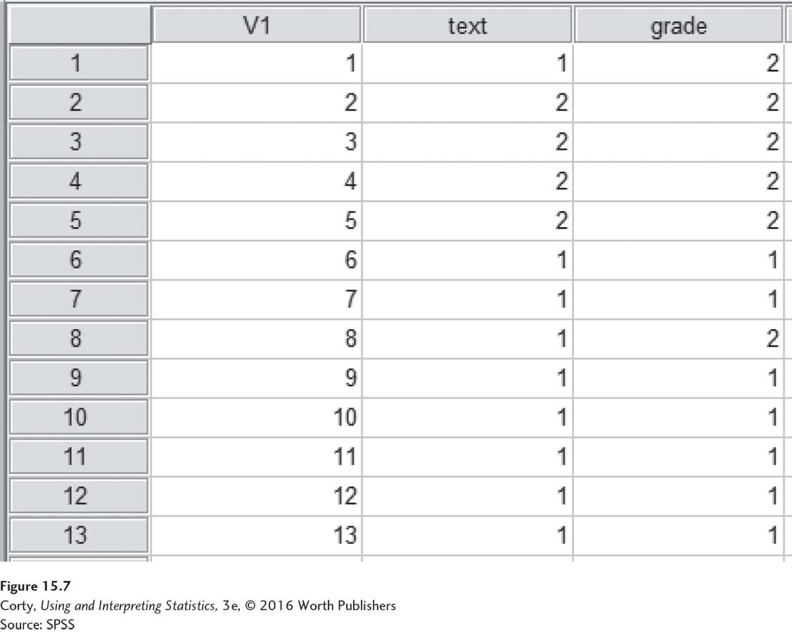
Data for a chi-square test of independence in SPSS are entered with each variable in a separate column and each case in a row. Figure 15.7 shows the data for the text-reading study. The second column, text, has a 1 if the student read the text before class and a 2 if the text was read after class. In the third column, grade, a 1 means a high grade (A or B) and a 2 means a low grade (C, D, or F).
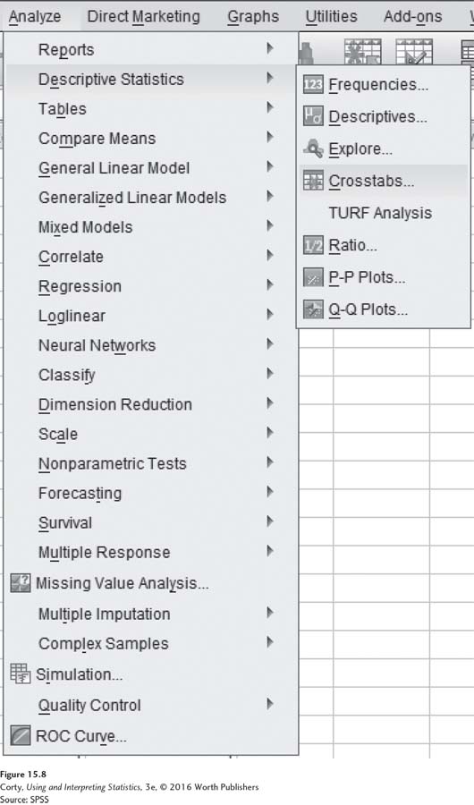
In SPSS, the chi-square test of independence is called “Crosstabs,” which is short for a cross-tabulation (contingency) table. Figure 15.8 shows that Crosstabs is located under “Analyze” and “Descriptive Statistics.”
Clicking on the Crosstabs command opens up the menu seen in Figure 15.9. Note that the variable “text” has already been sent over to be the row variable and the variable “grade” is getting ready to be sent to be the column variable. Be consistent—make the explanatory variable the row variable and the dependent variable the column variable.
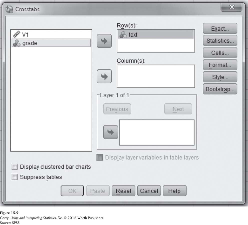
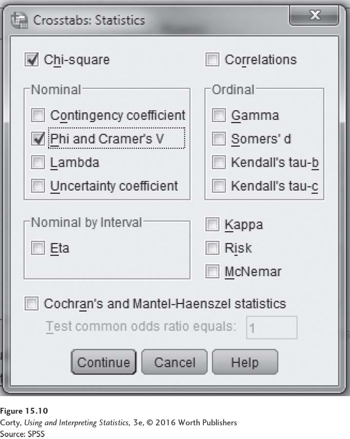
Clicking on the “Statistics” button in the upper-right-hand corner of Figure 15.9 opens the menu seen in Figure 15.10. Note that the boxes for “Chi-Square” and “Phi and Cramer’s V” have been checked. Then click on the “Continue” button in Figure 15.10 and the “OK” button in Figure 15.9.
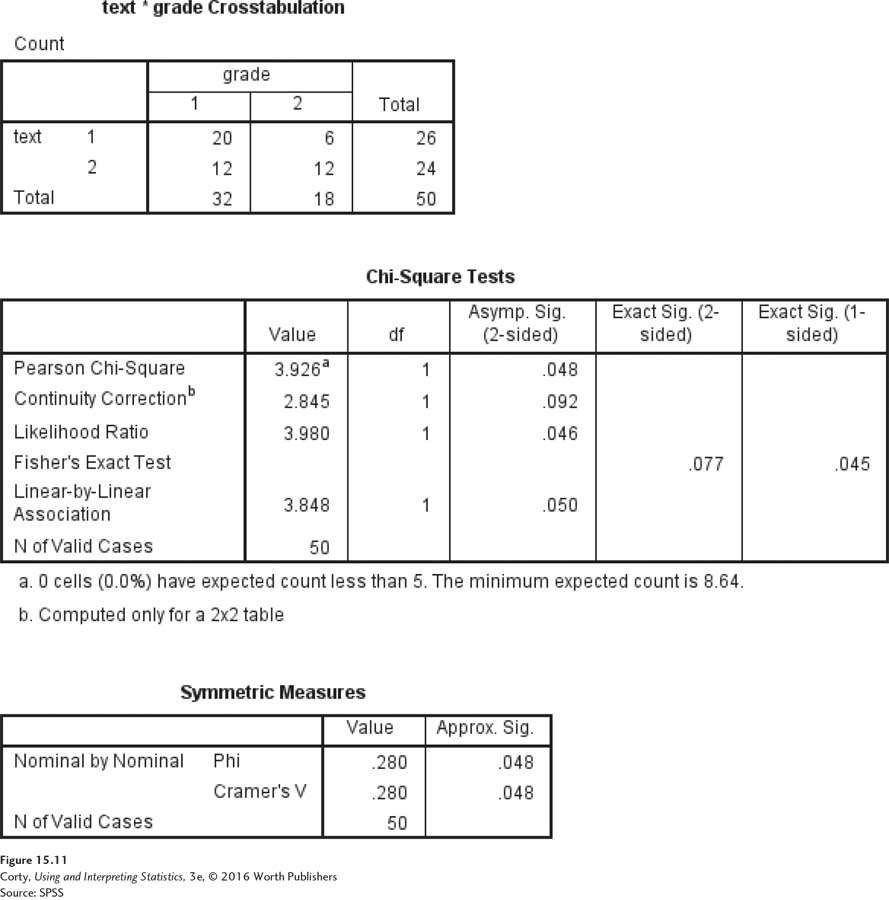
Once the statistics have been selected, clicking on the OK button on the crosstabs menu generates the output seen in Figure 15.11. The first box in the output (A) is the contingency table. The second box (B) gives the chi-square value, the degrees of freedom, and the exact significance level. SPSS calls chi-square “Pearson chi-square” and reports it on the first row as 3.926. Note that the subscript “a” means that all cells had expected frequencies greater than 5. The degrees of freedom are reported as 1 and the significance level as .048. If alpha is set at .05, then the results are statistically significant as long as the significance level is ≤.05. Finally, Cramer’s V is reported in the third box of the printout (C) as equal to .280.