Chapter 1 covered levels of measurement, classifying numbers as nominal, ordinal, interval, or ratio. Now let’s learn another way to classify numbers, as discrete or continuous. Knowing whether a number is discrete or continuous will be important in the next section of this chapter, which addresses how to graph a frequency distribution.

Discrete numbers answer the question “How many?” For example, the answers to questions like how many siblings one has, how many neurons are in a spinal cord, or how many jeans are in a closet are all discrete numbers. Discrete numbers take whole number values only and have no “in-between,” or fractional, values. No matter how raggedy a person’s favorite pair of jeans is, it’s still one pair of jeans. One would never say that a pair of jeans with a lot of holes is 0.79 of a pair of jeans. Nominal- and ordinal-level numbers are always discrete. Sometimes, interval- and ratio-level numbers are discrete.

Continuous numbers answer the question “How much?” For example, the answers to questions like how much aggression a person has, how much intelligence one has, or how much a person weighs would be continuous numbers. Continuous numbers can take on values between whole numbers, that is, they may have fractional values. The number of decimal places reported for continuous numbers, how specific they are, depends on the measuring instrument used. More precise measuring instruments allow attributes to be measured more exactly.

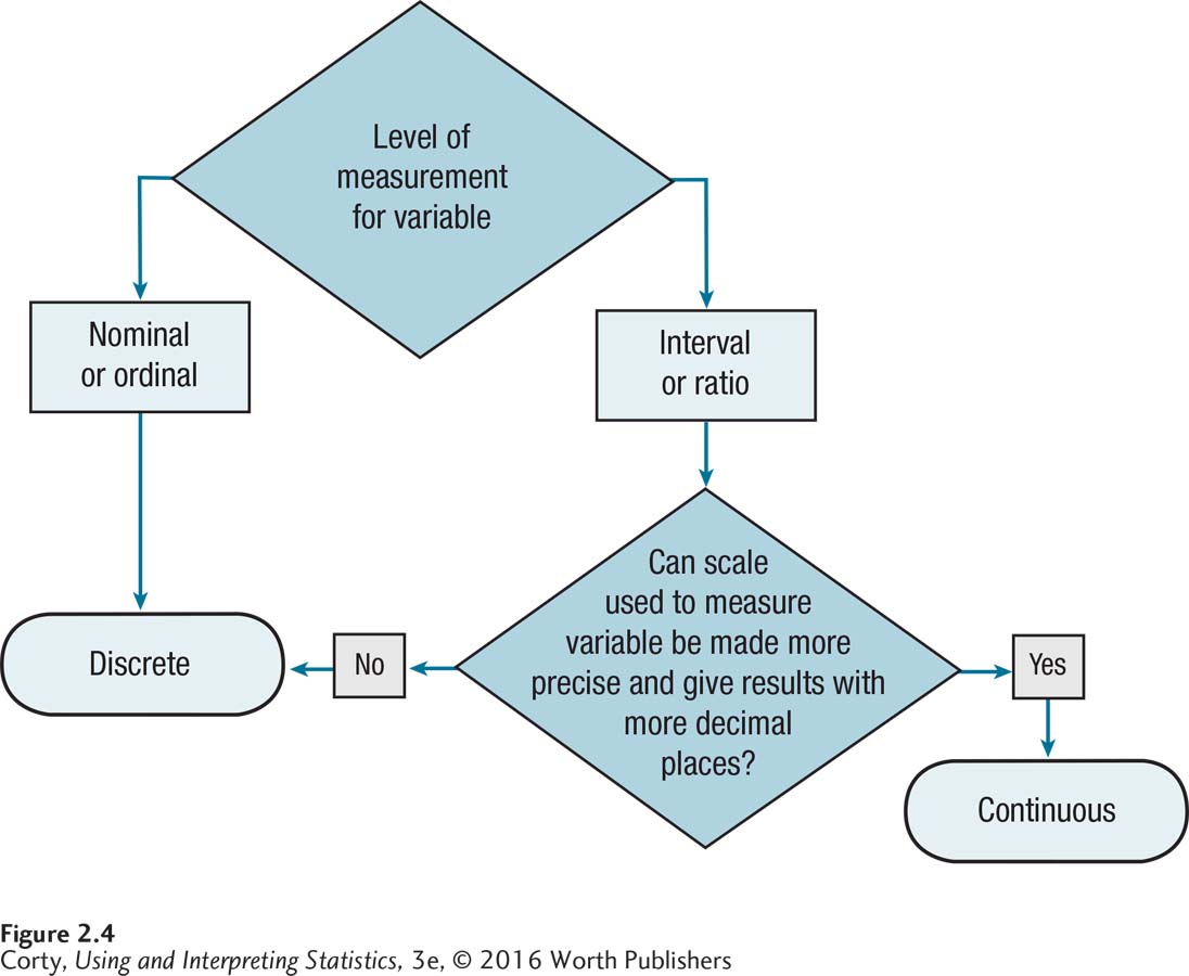
Because fractional values for continuous numbers represent distance, continuous numbers are always interval- or ratio-level numbers. Keep in mind, though, that not all interval- or ratio-level numbers are continuous. Figure 2.4 is a flowchart that leads one through the process of determining whether a number is discrete or continuous.

51

An example should make it clearer how continuous numbers can take on in-between values. Weight is a continuous number. Suppose Tyrone stepped on a digital scale, one that weighs to the nearest pound, and reported, “I weigh 175 pounds.” Does Tyrone weigh exactly 175 pounds? If there were a more precise scale, one that weighed to the nearest tenth of a pound, his weight might turn out to be 175.3 pounds. And, with an even more precise scale, one that measured to the nearest hundredth of a pound, his weight might now be found to be 175.34 pounds. How much Tyrone weighs depends on the precision of the scale used to measure him. Theoretically, continuous numbers can always be made more exact by using a better—more precise—measuring instrument.

52

Tyrone could weigh exactly 175 pounds, but he probably doesn’t. Statisticians think of his weight as falling within an interval that has a midpoint of 175. The question is this: How wide is the interval? How much or how little does Tyrone really weigh?

The answer is that Tyrone weighs somewhere from 174.5 to 175.5 pounds. The scale reports weight to the nearest pound, so the unit of measurement is 1 pound. Tyrone’s real weight falls somewhere in the interval from half a unit of measurement below his reported weight to half a unit of measurement above his reported weight. That’s from 175 – 0.5 = 174.5 to 175 + 0.5 = 175.5.

If Tyrone weighed less than 174.5, say, 174.2, then the scale would have reported his weight as 174, not 175 pounds. And if he weighed more than 175.5, say, 175.9, it would have reported his weight as 176 pounds. It is not clear where in the range from 174.5 to 175.5 his weight really falls, but his weight does fall in that range. His weight—a continuous number—is reported as the midpoint (175) of a range of values, any of which could be his real weight.

A single continuous number represents a range of values. To help understand this, think back to high school chemistry and measuring how acidic or basic a liquid was. This was done by dipping pH paper into the liquid and comparing the color of the pH paper to a key. An example of a key for pH is shown in Figure 2.5.

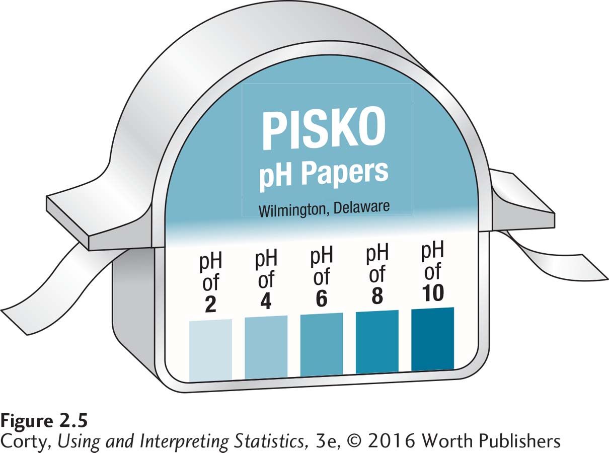
Suppose one dipped a piece of the pH paper from Figure 2.5 into a solution and it turned the shade associated with a pH of 6. Is the pH of the solution exactly 6? The pH is closer to 6 than to 4, or else the paper would have turned the lighter shade for 4. It is also closer to 6 than to 8, because the paper was not the darker shade for 8. The pH of the solution is closer to 6 than to 4 or 8, but it probably is not exactly 6.

In what range does the pH of the solution fall? This pH paper measures to the nearest 2 points so that is the unit of measurement. Half of the unit of measurement is 1, so subtracting that from 6 and adding it to 6 give the range within which the pH of the solution really falls: between 5 and 7. When this pH paper says 6, it really means somewhere between 5 and 7.

Those pH values, 5 and 7, are called the real limits of the interval. Real limits are the upper and lower bounds of a single continuous number or of an interval in a grouped frequency distribution for a continuous variable.

Table 2.10, the grouped frequency distribution of IQ for the 68 sixth graders, can be used to examine the real limits for an interval in a grouped frequency distribution. Here, IQ is measured to the nearest whole number. However, it would be possible to make a test that measures IQ to the nearest tenth or hundredth of a point, so IQ is a continuous variable. In Table 2.10, the bottom IQ interval ranges from 60 to 69, what are called the apparent limits for the interval. These are called apparent limits because they represent how wide the interval appears to be. But an IQ score of 60, at the bottom of the interval, really ranges from 59.5 to 60.5 and a score of 69, at the top of the interval, really ranges from 68.5 to 69.5. So, the scores in the 60 to 69 interval really fall somewhere in the range from 59.5, the real lower limit of the interval, to 69.5, the real upper limit. For continuous measures, real limits make researchers aware of how (im)precise their measures are.

53