4.3 Percentile Ranks
So far, the z score table in Appendix Table 1 has been used as it was designed. First, the z score is found in the table and then the area in the normal distribution is found above, below, or to that z score. Now, the table will be used to calculate percentile ranks.
A percentile rank tells the percentage of cases whose scores are at or below a given level in a frequency distribution. Percentile ranks provide a new way of thinking about a person’s score. Imagine a student, Leah, who obtained a score of 600 on an SAT subtest. (Remember, SAT subtests have a mean of 500 and a standard deviation of 100.) There have been two ways thus far of expressing Leah’s score: (1) as a raw score (X = 600), or (2) as a standard score (z = 1.00).
Here’s a third way, as a percentile rank. Using the z score of 1.00 and looking in column A of Appendix Table 1, 84.13% of the area under the normal curve falls at or below Leah’s score. Leah’s score as a percentile rank, abbreviated PR, is 84.13. Leah scored higher on this SAT subtest than about 84% of students. When her score is expressed in percentile rank form, it’s clear that Leah did well on this test.
Now let’s say that Joshua took the same test and his percentile rank was 2. Joshua didn’t do very well—he only performed better than 2% of other students. Comparing Leah to Joshua shows a major advantage of percentile ranks—they put scores into an easily interpretable context.
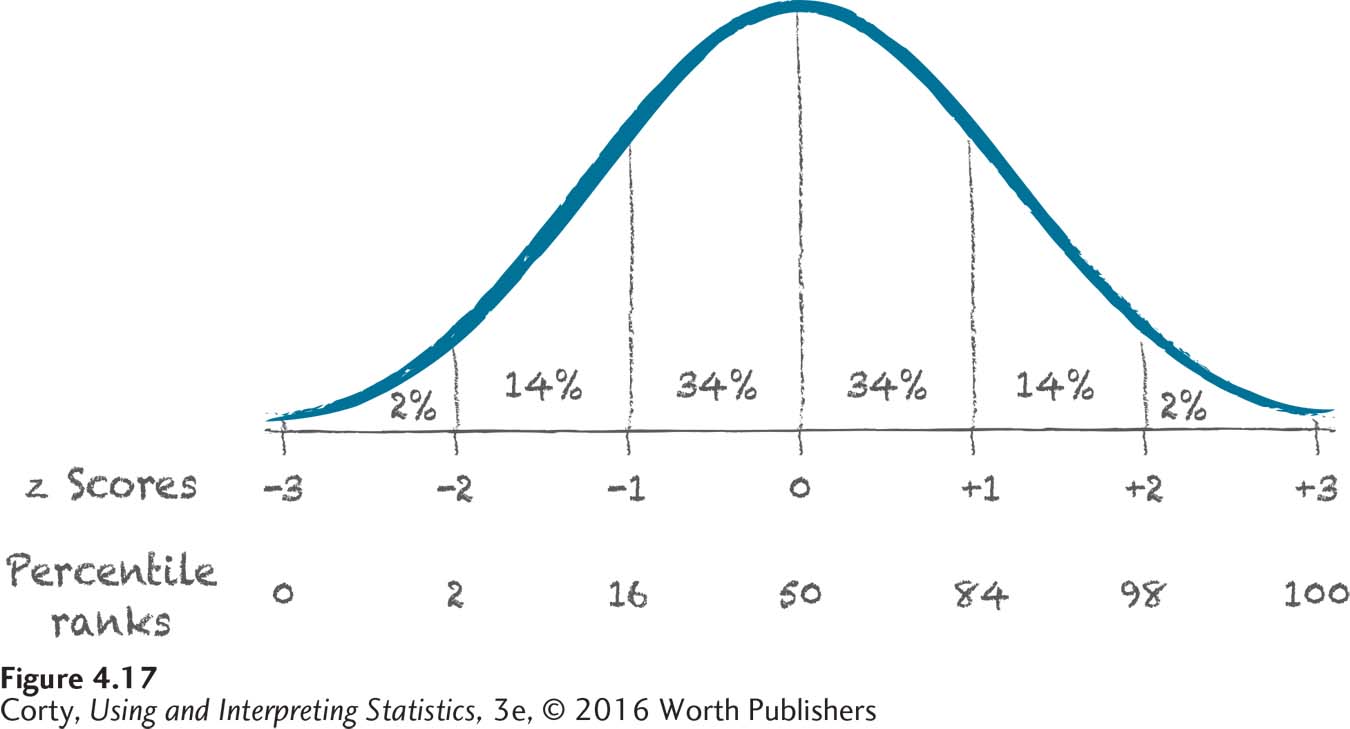
Figure 4.17 shows a normal distribution that is marked off (1) with the approximate percentages in each standard deviation (34%, 14%, and 2%), (2) with z scores (from –3 to +3) on the X-axis, and (3) with approximate percentile ranks, also on the X-axis. There are several things to note in this figure:

In this simplified version of the normal distribution, there are no cases that fall more than 3 standard deviations below the mean and none that fall more than 3 standard deviations above it.
This means that the percentile rank associated with a z score of –3 is 0, and the percentile rank associated with a z score of +3 is 100.
Page 125The midpoint is the median. This means that a score at the midpoint has a percentile rank of 50.
≈2% of cases fall from the bottom of the normal curve to z = –2, so the percentile rank for z = –2 is 2.
Moving up the normal distribution, it’s clear that percentile ranks grow as one moves to the right along the X-axis.
A Common Question
Q What is the level of measurement for percentile ranks?
A Percentile ranks don’t have equality of units, so they are ordinal. Look at Figure 4.16 and note that the distance (in z score units) from a PR of 2 to a PR of 16 is the same as the distance from a PR of 16 to a PR of 50. In one case, a single z score covers 14 PR units and in the other it covers 34 PR units.
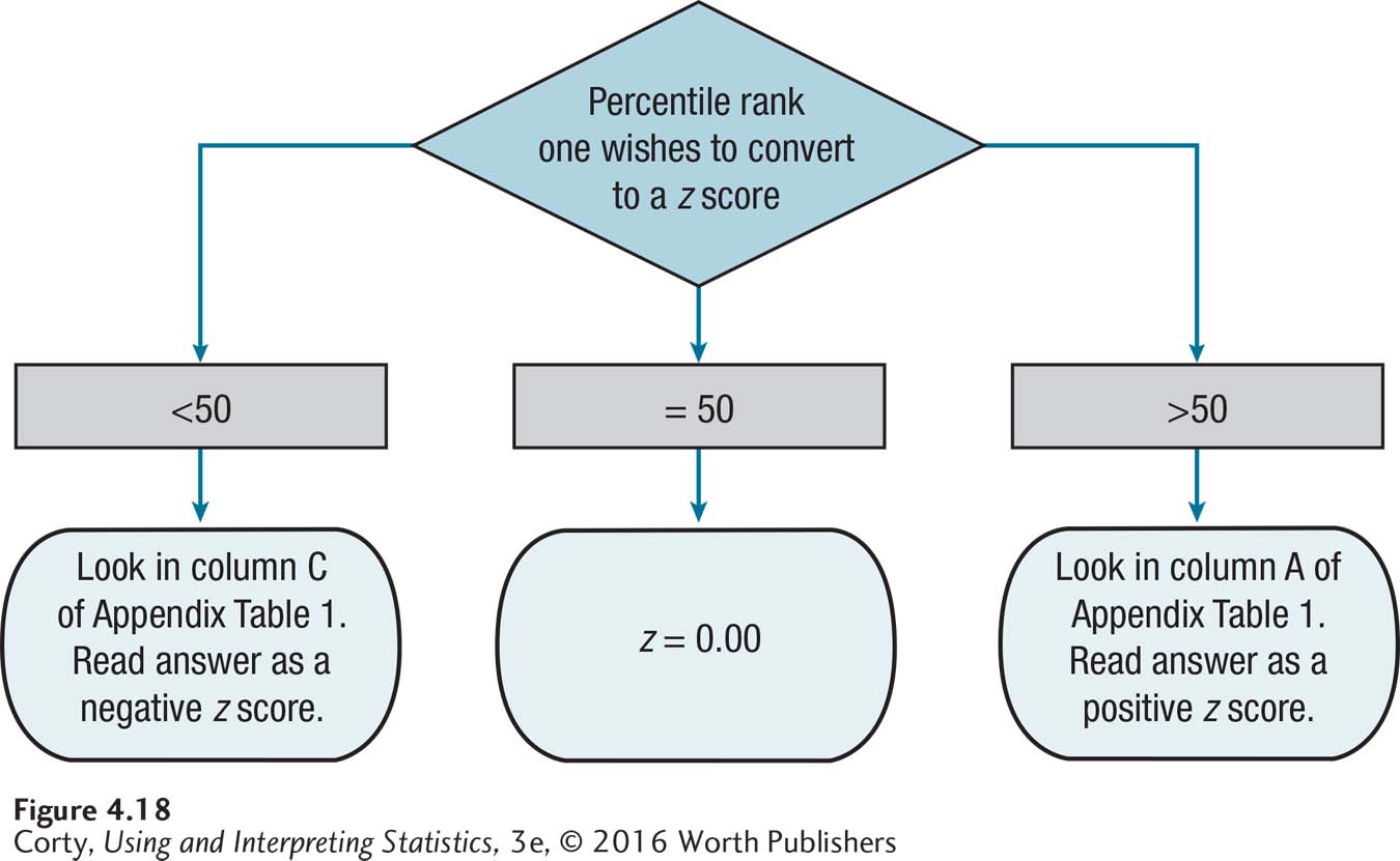
A percentile rank can be calculated from a raw score or a z score. Alternatively, a raw score or a z score can be calculated from a percentile rank by using Appendix Table 1. The flowchart in Figure 4.18 shows how to do this.

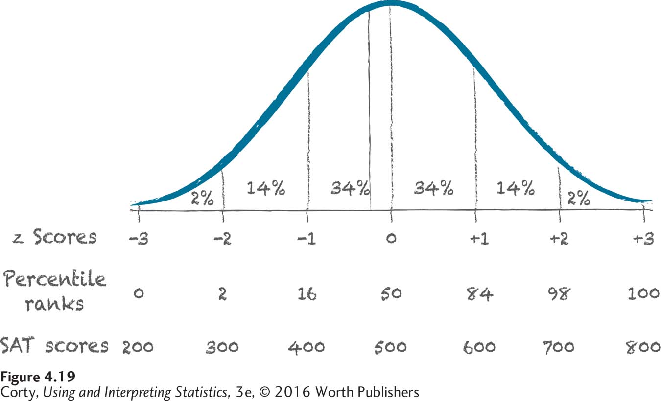
Imagine another student, Kelli, who took the same SAT subtest and whose score had a percentile rank of 40. What is her z score? A sketch always helps. Figure 4.19 shows a normal distribution. The X-axis is marked with z scores, percentile ranks, and SAT subtest scores, which shows how these three scores are equivalent. For example, a z score of 1 is equivalent to a percentile rank score of 84 and an SAT subtest score of 600. There is also an X on the X-axis about where a percentile rank of 40 would be. The X shows that this percentile rank will have an associated z score that falls somewhere between –1 and 0 and an associated SAT score that falls somewhere between 400 and 500.

Now, it is time to calculate Kelli’s z score more exactly. According to the flowchart in Figure 4.18, to find the z score associated with a percentile rank less than 50, go to column C in Appendix Table 1, which shows that the z score will be negative. Move down column C. The row closest to a value of 40.00 shows a z score of 0.25. This score needs to be treated as a negative number, so the answer is –0.25. Kelli’s grade on the test, as a z score, is –0.25.
Kelli’s grade is now known in two formats: as a percentile rank (40) and as a z score
(–0.25). What is her score as a raw score on the SAT subtest? To answer that question, use Equation 4.3:
X = 500 + (–0.25 × 100)
= 500 + (–25.0000)
= 500 – 25.0000
= 475.0000
= 475.00
Kelli obtained a 475.00 on this SAT subtest.
Worked Example 4.3
Imagine that Clayton takes an IQ test, with a mean of 100 and a standard deviation of 15, and does better than 95% of the population. If he did better than 95%, then his score, as a percentile rank, is 95. What was his IQ score if his score was a 95 as a percentile rank?
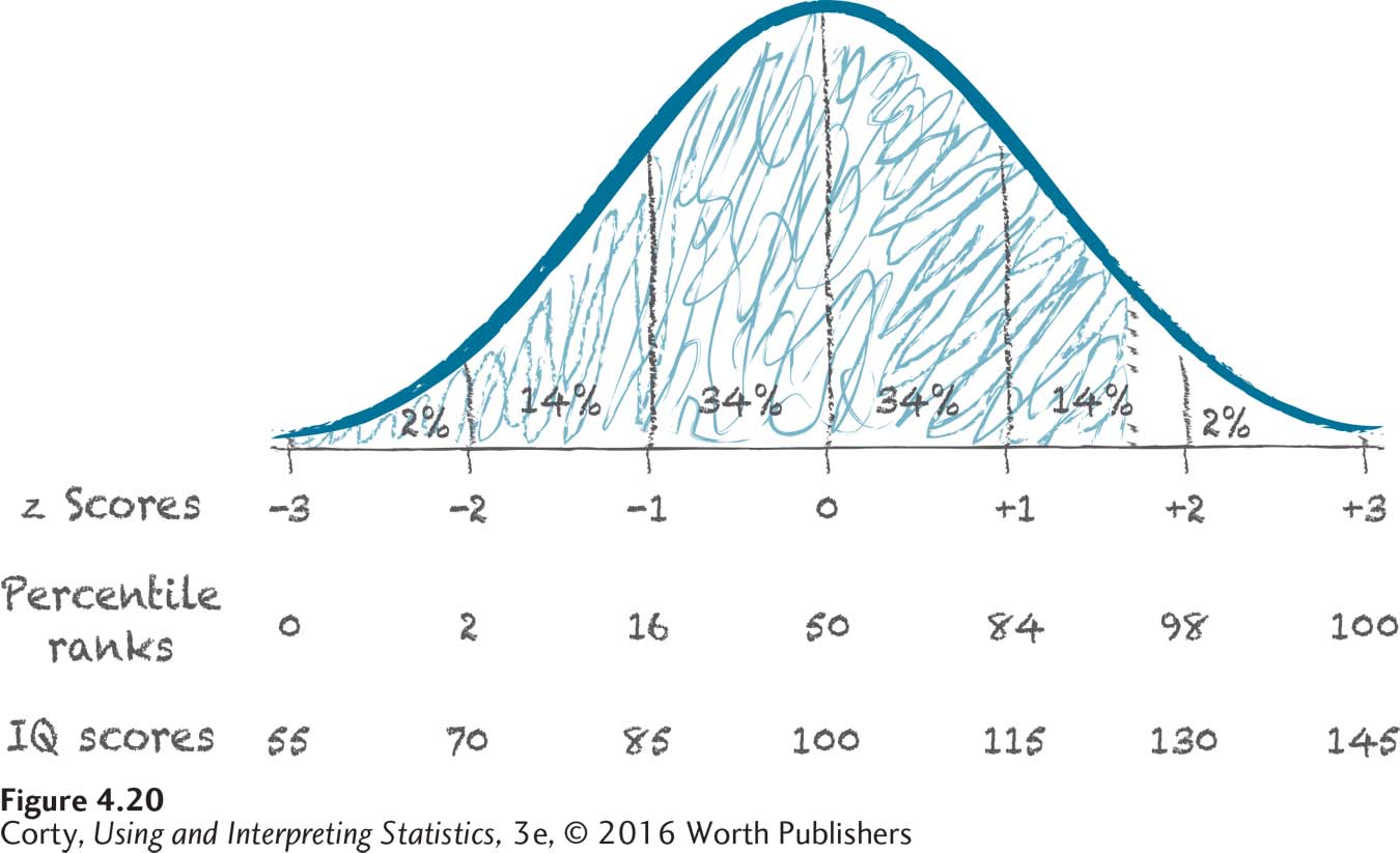
First, make a sketch. In Figure 4.20, the X-axis is marked with z scores, percentile ranks, and IQ scores and a dotted line is drawn about where PR 95 should be. The line is between z scores of 1 and 2, closer to 2 than to 1. In IQ units, it is between 115 and 130, closer to 130.

To calculate the raw score, use the flowchart in Figure 4.18. Clayton’s score has a percentile rank above 50, so turn to column A of Appendix Table 1. In that column, look for the value closest to 95%. In this case, there are two values, 1.64 and 1.65, that are equally close to 95.00. Logic can be used to decide which of these to select:
A z score of 1.64 is higher than 94.95% of scores. This doesn’t quite capture the 95% value that is Clayton’s score.
A z score of 1.65 is higher than 95.05% of scores. This captures the 95% value that is Clayton’s score.
To select the score that is as good or better than 95% of the cases in a normal distribution, go with 1.65. Clayton’s score, as a z score, is 1.65.
To convert that z score to an IQ score, use Equation 4.3:
XIQ = 100 + (1.65 × 15)
= 100 + 24.7500
= 124.7500
= 124.75
Clayton’s score on the IQ test is 124.75, a score that was better than that of 95% of the population.
Remember the angioplasty graph from the beginning of the chapter? It showed that most cities had “normal” rates of angioplasty and one city was unusually high. Let’s see how unusual that city is.
To do so, we need to know the mean angioplasty rate for the sample of cities (11) and the standard deviation (4). This allows us to calculate a z score for the outlier city that has an angioplasty rate of 42:

This city has an angioplasty rate that is 7.75 standard deviations above the national average. This is a very extreme score. The z score table in the back of the book only goes up to a z score of 5.00; and “only” 0.00003% of cases fall above this. A score of 7.75 is farther out in the tail than this, so it is an incredibly rare event. To a statistician’s mind, such extreme events don’t just happen by chance. There’s something fishy going on in that city, something that has inflated the rate at which angioplasties are performed.
Practice Problems 4.3
Review Your Knowledge
4.12 What is a percentile rank?
4.13 What is the percentile rank for a score at the midpoint of a set of normally distributed scores?
Apply Your Knowledge
4.14 If a person’s score, as a percentile rank, is 80, what is her z score?
4.15 What is the percentile rank associated with a z score of –0.45?