Now that we have examined the output and entry and exit decisions for firms in a competitive market, we can derive the industry supply curve, which you have been working with since Chapter 3. Supply curves can slope upward, be flat, or in rare circumstance even slope downward. We will show that the slope of the supply curve can be explained by how costs change as industry output increases or decreases.

In an increasing cost industry, costs increase with greater industry output and this generates an upward-sloping supply curve. In a constant cost industry, costs do not change with changes in industry output and this generates a flat supply curve. In a decreasing cost industry, costs decrease with greater industry output and this generates a downward-sloping supply curve. Decreasing cost industries are rare.

Let’s start with increasing cost industries.

207

In an increasing cost industry, costs rise as industry output increases. The oil industry is an increasing cost industry because greater quantities of oil can be produced only by using more expensive methods such as drilling deeper, drilling in more inhospitable spots, or extracting the oil from tar sands.

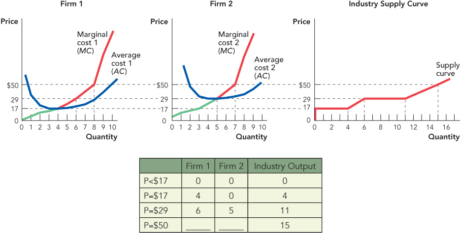
To illustrate, let’s focus on just two firms. Firm 1 is the firm that we examined earlier. Its oil is located near the surface, so its average costs are low and it enters the industry when the price of oil rises to just $17. Firm 2’s oil, however, is located deeper than Firm 1’s, and so Firm 2’s fixed costs of drilling are higher and its average cost curve is higher than that of Firm 1. As a result, Firm 2 will not enter the industry until the price of oil reaches $29. We can now build the industry supply curve.

At any price below $17, what is the quantity supplied? Zero. At a price less than $17, the firm is losing money so no firm enters the industry, and the industry supply curve, indicated in the rightmost panel of Figure 11.7 by the red line, shows a quantity supplied of zero. When the price of oil hits $17, Firm 1 enters the industry at its profit-maximizing quantity of 4 barrels and thus industry supply at a price of $17 jumps to 4 barrels. As the price rises, Firm 1 expands along its MC curve and so does industry supply. When the price hits $29, Firm 2 enters the industry with its profit-maximizing quantity of 5 barrels of oil. To find the quantity supplied by the industry, we sum the quantity supplied by each firm in the industry. At a price of $29, Firm 1 supplies 6 barrels of oil and Firm 2 supplies 5 barrels of oil, so industry supply is 11 barrels of oil. As the price rises further, both firms now expand along their respective MC curves. Once again, industry supply at any price is found by adding up the quantity supplied by each firm at that price. Thus at a price of $50, Firm 1 produces 8 barrels of oil and Firm 2 produces 7 barrels of oil, so industry supply at a price of $50 is 15 barrels of oil.

208

Our explanation of the supply curve is simply a more detailed version of the account in Chapter 3. At a low price, the only oil that is profitable to exploit is the oil that can be recovered at low cost from places like Saudi Arabia. As the price of oil rises, it becomes profitable to supply oil from the North Sea, the Athabasca tar sands, and other higher-cost sources. The analysis in Chapter 3 focused on how a higher price encourages entry from higher-cost producers. This chapter adds to the entry story the idea that as the price increases, each firm expands output by moving along its marginal cost curve.

More generally, any industry that buys a large fraction of the output of an increasing cost industry will also be an increasing cost industry. The gasoline industry, for example, is an increasing cost industry because greater demand for gas will push up the price of oil, which in turn increases the price of gas. The electricity industry is an increasing cost industry because greater demand for electricity pushes up the price of coal, and coal is an increasing cost industry for the same reasons as oil.

Consider the industry of domain name registrars. Web pages on the Internet have a conventional name, called a domain name, such as that for the National Bureau of Economic Research, which has the domain name NBER.org. But the conventional names are just masks for more difficult-to-remember numbers called IP (Internet Protocol) addresses. When you type www.NBER.org into a browser, the browser sends a message to the Domain Name System (DNS), which looks up and returns the corresponding IP address, in this case http://199.233.228.243/. The IP address tells your browser where to find the information that is posted by the NBER. So, in order to work, every domain name must be registered with the DNS and assigned an IP address. Domain name registrars are firms that manage and register domain names.

The domain name registration industry has two important characteristics. First, domain name registration satisfies all of the conditions for a competitive industry.

The product being sold is similar across sellers.

There are many buyers and sellers, each small relative to the total market.

There are many potential sellers.

As far as the user is concerned, there is little difference between registering with GoDaddy.com or GetRealNames.com so the product is similar across sellers. There are many buyers and many sellers. There are hundreds of registrars in the United States alone. Indeed, GoDaddy.com is based in the United States and GetRealNames.com is based in India; thus, there is worldwide trade in domain name registration. Furthermore, not only are there many competitors in the industry, but just about anyone in the world can become an accredited registrar with an investment of a few thousand dollars, so there are many potential competitors.

209

The second important characteristic of the domain name industry is that the major input for domain name registration is a bank of computers, but all the computers of all the domain name registrars in all the world don’t add up to much compared with the world supply of computers. The domain name industry, therefore, can expand without pushing up the prices of its major inputs and thus without raising its own costs. An industry that can expand or contract without changing the prices of its inputs is called a constant cost industry.

These two characteristics, free entry and the fact that the industry demands only a small share of its major inputs, produce the following properties: (1) The price for domain name registration is quickly driven down to the average cost of managing and assigning a domain name, so profits are quickly driven to normal levels; and (2) because average costs don’t change much when the industry expands or contracts, the price of domain name registration doesn’t change much when the industry expands or contracts so the long-run supply curve is very elastic (flat).

Let’s examine these characteristics in turn. One of the largest registrars is GoDaddy.com, which charges $6.99 to register a domain name for one year. What would happen if it raised its price to $14.95 a year? GoDaddy would quickly lose a significant fraction of its business. New customers would choose other firms, and since domains must be renewed every few years, old customers would soon also switch. As a result of this competition, GoDaddy and every other firm in the industry price their services at near average cost and earn a zero or normal profit.

Now consider what happens when the demand for domain names increases. In 2005, there were more than 60 million domain names. Just one year later, there were more than 100 million domain names. If the demand for oil nearly doubled, the price of oil would rise dramatically, but despite nearly doubling in size, the price of registering a domain name has not increased. When an increase in demand hits a constant cost industry, the price rises in the short run as each firm moves up its MC curve. But the expansion of old firms and the entry of new firms quickly push the price back down to average cost.

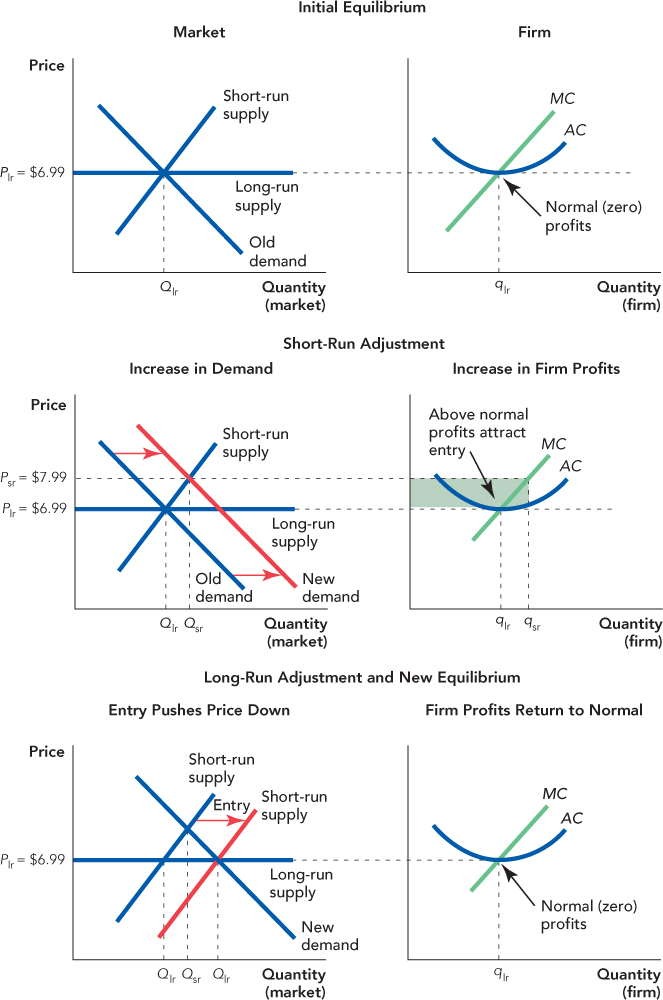
Figure 11.8 illustrates how a constant cost industry responds to an increase in demand. The figure looks imposing, but if we consider it in steps, the logic of the story will be clear. In the top panel, we have the initial equilibrium. On the left-hand side of the panel, we illustrate the industry. The market price is P_lr ($6.99 in the case of domain name registration), the market quantity is Q _lr, and the quantity demanded is exactly equal to the quantity supplied so the industry is in equilibrium. On the right-hand side of the panel, we have a typical firm in the industry. The firm is profit-maximizing because P = MC and it is making a zero or normal profit because P = AC. Note that the industry output is Q _lr but the firm output is q _lr, which indicates that each firm in the industry produces only a small share of total industry output.

In the middle panel on the left, we illustrate an increase in demand from Old demand to New demand. In the short run, the increase in demand increases price to P_sr, $7.99, where New demand and Short-run supply meet. The industry quantity increases to Q_sr. Where does the increase in quantity come from? It comes from many firms in the industry, each of which produces a little bit more by increasing production along its MC curve. In the middle panel on the right, we show that the typical firm in the industry expands to q_sr, and since the price is above average cost, the firm earns profits as illustrated by the shaded area (P – AC) × q_sr.

210

211

Before turning to the bottom panel, let’s remember that the short run is the period before entry (or exit) occurs. In the middle panel, we are illustrating the first response to an increase in demand, which is that the price rises and every firm in the industry responds by increasing production along its marginal cost curve. (Indeed, the short-run supply curve is simply the sum of the MC curves for each firm in the industry.)

The increase in price generates above-normal profits for each firm in the industry. Notice that above-normal profits attract new investment and entry. Entry is the second response to the increase in demand. In some industries, like the domain name registration industry, entry might take a matter of a few months or even as little as a few weeks, while in other industries it could take several years before significant entry occurs.

When entry does occur, the short-run supply curve shifts to the right, and as it does, the price falls and profits are reduced. Entry doesn’t stop until profits return to normal levels so entry continues until price is pushed down to AC. In the long run, after all entry and exit have occurred, profits have returned to normal.

Since the prices of the industry inputs don’t change when the industry expands, the AC curve of each firm in the industry doesn’t change, so in the new industry, equilibrium price is again equal to P_lr, $6.99. Although the typical firm produces q _lr, just as it did before the increase in demand, the industry quantity has increased to Q _lr because there are now more firms in the industry.

Thus, the key to a constant cost industry is that it is small relative to its input markets, so when the industry expands, it does not push up the price of its inputs and thus industry costs do not increase.

In an increasing cost industry, firm costs increase as the industry expands, and thus, the supply curve slopes upward. In a constant cost industry, firm costs are constant as the industry expands, and thus, the long-run supply curve is flat. Could firm costs decrease as the industry expands, creating a decreasing cost industry with a downward-sloping supply curve? Yes. To see how, we must ask the question: Why is Dalton, Georgia, the “carpet capital of the world”?

An amazing 72% of the $12 billion worth of carpets produced in the United States every year are produced in Dalton and the surrounding area. Dalton is home to 150 carpet plants and hundreds of machine shops, cotton mills, dye plants, and other related industries. Why Dalton? Dalton is not like Saudi Arabia, as it has no outstanding natural advantages for producing carpets, so why is Dalton the carpet capital of the world? The answer is nothing more than an accident of history that launched a virtuous circle.

The Dalton carpet industry began in 1895 with one teenage girl who crafted an especially beautiful bedspread for her brother’s wedding. Wedding guests saw the bedspread and asked her to make more. To meet the demand, she hired workers and trained them in her innovative techniques. As demand grew even further, these workers and others went into business for themselves, creating a bedspread industry. The skills needed to make bedspreads were also useful for making carpets, so carpet firms began to locate in Dalton. With so many carpet firms located in Dalton, it became profitable to open trade schools to teach carpet-making skills. In turn, the trade schools made it even more cost-efficient for carpet firms to move to Dalton. Similarly, machine shops, cotton mills, and dye plants moved to Dalton to be close to their customers, and the ready access to machine shops, cotton mills, and dye plants made it even less costly for carpet firms to make carpets in Dalton. The resulting virtuous circle made Dalton the cheapest place to make carpets in the United States—not because Dalton had natural advantages but because it was cheaper to make carpets in a place where there already were a lot of carpet makers.

212

Decreasing cost industries are important, but very special because costs cannot decrease forever. Dalton became the cheapest place to produce carpets in the United States many years ago and that is unlikely to change any time soon. But if the demand for carpets were to increase today, the cost of making carpets in Dalton would increase, not fall further. The cost of making carpets in Dalton fell when the local industry expanded from 1 to 50 firms, but they didn’t fall by nearly as much when the industry expanded from 50 to 100 firms.

Economists use the idea of a decreasing cost industry to explain the history of industry clusters: not just carpets in Dalton, Georgia, but computer technology in Silicon Valley, movie production in Hollywood, and flower distribution in Aalsmeer, Holland. Once the cluster is established, however, constant or increasing costs are the norm. If the demand for carpet were to increase today, for example, the price of carpets would rise, not fall.

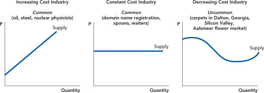
In an increasing cost industry, costs increase with industry output and the supply curve slopes upward. If the industry is small relative to its input markets so the industry can expand without pushing up its costs, the supply curve will be flat; we call this a constant cost industry. Industry supply curves can even slope downward but this is rare and temporary, although the idea of a decreasing cost industry is important for explaining the existence of industry clusters. Figure 11.9 illustrates the three possibilities.

213