Governments are not the only source of market power. Monopolies can arise naturally when economies of scale create circumstances where one large firm (or a handful of large firms) can produce at lower cost than many small firms. When a single firm can supply the entire market at lower cost than two or more firms, we say that the industry is a natural monopoly.

A subway is a natural monopoly because it would cost twice as much to build two parallel subway tunnels than to build one, but even though costs would be twice as high, output (the number of subway trips) would be the same. Utilities such as water, natural gas, and cable television are typically natural monopolies because in each case it’s much cheaper to run one pipe or cable than to run multiple pipes or cables to the same set of homes.

In Figure 13.5, we compared competitive firms with an equal cost monopoly and showed that total surplus was higher under competition. The comparison between competitive firms and natural monopoly is more difficult. Even though natural monopolies produce less than the optimal quantity, competitive firms would also produce less than the optimal quantity because they could not take advantage of economies of scale.

If the economies of scale are large enough, it’s even possible for price to be lower under natural monopoly than it would be under competition. Figure 13.6 shows just such a situation. Notice that the average cost curve for the monopoly is so far below the average cost curves of the competitive firms, that the monopoly price is below the competitive price. It’s possible, for example, for every home to produce its own electric power with a small generator or solar panel, but the costs of producing electricity in this way would be higher than buying electricity produced from a dam even if the dam was a natural monopoly.

246

Is there any way to have our cake and eat it too? That is, is there a way to have prices equal to marginal cost and to take advantage of economies of scale?

In theory the answer is yes, but it’s not easy. In Chapter 8, we showed that a price control set below the market price would create a shortage. But surprisingly, when the market price is set by a monopolist, a price control can increase output. Let’s see how.

Suppose that the government imposes a price control on the monopolist at level P_R, as in Figure 13.7. Imagine that the monopolist sells two units and suppose it wants to sell a third. What is the marginal revenue on the third unit? It’s just P_R. In fact, when the price is set at P_R, the monopolist can sell up to Q_R units without having to lower the price. Since the monopolist doesn’t have to lower the price to sell more units, the marginal revenue for each unit up to Q_R is P_R. Notice that we have drawn the new marginal revenue curve in Figure 13.7 equal to P_R in between 0 and Q_R (after that point, to sell an additional unit, the monopolist has to lower the price on all previous units so the MR curve jumps down to the level of the old MR curve and becomes negative). Now the problem is simple because, as always, the monopolist wants to produce until MR = MC, so Q_R is the profit-maximizing quantity.

Notice that the monopolist produces more as the government-regulated price of its output falls.

So what price should the government set? Since the optimal quantity is found where P = MC, the natural answer is that the government should set P_R = MC. Unfortunately, that won’t work when economies of scale are large because if the price is set equal to marginal cost, the monopolist will be taking a loss. Remember that Profit = (P – AC) × Q so setting P_R equal to marginal cost creates a loss illustrated by the red area in Figure 13.7.

The government could subsidize the monopolist to make up for the loss when P_R = MC but, once again, taxation has its own deadweight losses. If the government set P_R = AC at point a, where the AC curve intersects the demand curve, the monopolist would just break even; output would then be larger than the monopoly quantity but less than the optimal quantity. This seems like a fairly good solution, but there are other problems with regulating a monopolist. When the monopolist’s profits are regulated, it doesn’t have much incentive to increase quality with innovative new products or to lower costs. The strange history of cable TV regulation and California’s ill-fated efforts at electricity deregulation illustrate some of the real problems with regulating and deregulating monopolies.

247

Regulation of retail subscription rates for cable TV seemed to keep prices low in the early years of television, when there were basically only three channels, ABC, CBS, and NBC. In the 1970s, however, new technology made it possible for cable operators to offer 10, 20, or even 30 channels. But if subscription rates were fixed at the low levels, thereby limiting profit rates, the cable operators would have little incentive to add channels. Recognizing this, Congress lifted caps on pay TV rates in 1979 and on all cable television in 1984.

Deregulation of cable TV rates led to higher prices, just as the theory of natural monopoly predicts, but something else happened—the number of television channels and the quality of programming increased dramatically. And, contrary to natural monopoly theory, consumers seemed to appreciate the new channels more than they disliked the higher prices. This is evident because even as prices rose, more people signed up for cable television.12

Congress re-regulated “basic cable” rates in 1992 but left “premium channels” unregulated. Wayne’s World was the result. Let’s explain: Cable operators were typically required to carry a certain number of channels in the basic package, but they had some choice over which channels were included in the package. So when basic cable was re-regulated, the cable operators moved some of the best channels to their unregulated premium package. To fill the gaps in the basic package, they added whatever programs were cheap, including television shows created by amateurs on a shoestring budget. Wayne’s World, a Saturday Night Live comedy sketch, mocked the proliferation of these amateur cable shows.

248

Rates were mostly deregulated again in 1996. Not entirely coincidentally, this was the first year that HBO won an Emmy. Today, “basic tier cable” is regulated by local governments, but anything beyond the most basic service is predominantly free of regulation and cable companies can charge a market rate. As before, prices have risen since deregulation, but so have the number of television channels and the quality of programming.

If you like Game of Thrones, Pretty Little Liars, and The Walking Dead, then cable deregulation has worked well. Deregulation of electricity, however, has proven shocking.

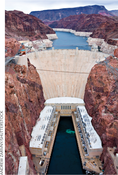
Government ownership is another potential solution to the natural monopoly problem. In the United States, there are some 3,000 electric utilities, and two-thirds of them are government-owned (the remainder are heavily regulated). Government ownership of utilities began early in the twentieth century with municipalities owning local distribution companies. In the 1930s, the federal government became a major generator of electricity with the construction of the then largest manmade structures ever built, the Hoover Dam in 1936 and the even larger Grand Coulee Dam in 1941.

Government ownership and regulation worked reasonably well for several decades in providing the United States with cheap power. Without the discipline of competition or a profit motive, however, there is a tendency for a government-run or regulated monopoly to become inefficient. Why reduce costs when costs can be passed on to customers? In the 1960s and 1970s, multi billion-dollar cost overruns for the construction of nuclear power plants drew attention to industry inefficiencies as the price of power increased.

Historically, a single firm handled the generation, long-distance transmission, and local distribution of electricity. In the 1970s, however, new technologies reduced the average cost of generating electricity at small scales (in Figure 13.6 you can think of the curves labeled “Average costs for small firms” as moving down). Although the transmission and distribution of electricity remained natural monopolies, the new technologies meant that the generation of electricity was no longer a natural monopoly. Economists began to argue that unbundling generation from transmission and distribution could open up electricity generation to competitive forces, thereby reducing costs.

Hoping to benefit from lower costs and greater innovation, California deregulated wholesale electricity prices in 1998. In the first two years after deregulation, all appeared well. In fact, as the new century was born, California was booming. In Silicon Valley, college students in computer science were being turned into overnight millionaires and billionaires. In 2000, personal income in California rose by a whopping 9.5%. Higher incomes and an unusually hot summer increased the demand for electricity. But California’s generating capacity, which was old and in need of repair, began to strain. To meet the demand, California had to import power from other states, but other states had little to spare. Hot weather was pushing up demand throughout the West and the supply of hydro-electric power had fallen by approximately 20% because of low snowfall the previous winter.

249

All of these forces and more smashed together in the summer of 2000 to double, triple, quadruple, and finally quintuple the wholesale price of electricity from an average in April of $26 per megawatt hour (MWh) to an August high of $141 per MWh. Prices declined modestly in the fall but jumped again in the winter, reaching for one short period a price of $3,900 per MWh and peaking in December at an average monthly price of $317 per MWh—about 10 times higher than the previous December’s rate.13 Worse yet, when not enough power was available to meet the demand, blackouts threw more than 1 million Californians off the grid and into the dark. The new century wasn’t looking so bright after all.

Mother Nature was not the only one to blame for California’s troubles. The combination of increased demand, reduced supply, and a poorly designed deregulation plan had created the perfect opportunity for generators of electricity to exploit market power.

When the demand for electricity is well below capacity, each generator has very little market power. If a few generators had shut down in 1999, for example, the effect on the price would have been minimal because the power from those generators could easily have been replaced with imports or power from other generators. Thus, in 1999, each generator faced an elastic demand for its product. In 2000, however, every generator was critical because nearly every generator needed to be up and running just to keep up with demand. Electricity is an unusual commodity because it is expensive to store, and if demand and supply are ever out of equilibrium, the result can be catastrophic blackouts. Thus, when demand is near capacity, a small decline in supply leads to much higher prices as utilities desperately try to buy enough power to keep the electric grid up and running. Thus, in 2000, the demand curve facing each generator was becoming very inelastic. And what happens to the incentive to increase price when demand becomes inelastic? Do you remember the lesson of Figure 13.4, also pictured on the right in Figure 13.8?

In the summer and winter of 2000, demand was near capacity and every generator was facing an inelastic demand curve. A firm that owned only one generating plant couldn’t do much to exploit its market power: If it shut down its plant, the price of electricity would rise but the firm wouldn’t have any power to sell! Many firms, however, owned more than one generator, and in 2000, this created a terrible incentive. A firm with four generators could shut down one, say, for “maintenance and repair,” and the price of electricity would rise by so much that the firm could make more money selling the power produced by its three operating generators than it could if it ran all four! Suspiciously, far more generators were taken off-line for “maintenance and repair” in 2000 and early 2001 than in 1999.14

250

California was not the only state to restructure its electricity market in the late 1990s. Other states such as Texas and Pennsylvania had opened up generation to competition and have seen modestly lower electricity prices. Restructuring has also occurred in Britain, New Zealand, Canada, and elsewhere, but California’s experience has demonstrated that unbundling generation from transmission and distribution, which remain natural monopolies, is tricky.