The Budget Constraint
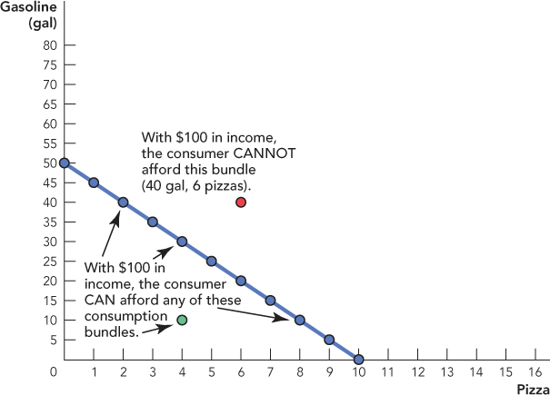
Imagine that there are only two goods as before, but just for variety, we will switch to gasoline and pizza. Gasoline is $2 per gallon and pizzas are $10 apiece. Let’s suppose also that the consumer has $100 of income. Figure 25.4 shows the consumer’s budget constraint, namely all of the bundles of gasoline and pizza that the consumer can afford given his income and prices. For example, the consumer could buy 50 gallons of gas and 0 pizzas, or 10 pizzas and 0 gallons of gas, or any consumption bundle along the line connecting these two points. The consumer cannot afford bundles that are “outside” the budget constraint. For example, the consumer cannot afford the red bundle of 40 gallons and 6 pizzas. (How much income would the consumer need to afford this bundle?)

A budget constraint shows all the consumption bundles that a consumer can afford given their income and prices.
470
In addition to the points along the budget constraint, the consumer can also afford any point that is “inside” the budget constraint, such as the green point of 10 gallons and 4 pizzas. If the consumer bought this bundle of goods, however, he would spend $60 ($2 × 10 + $10 × 4), leaving him with $40 in income. Note, however, that in this model, there are only two goods and no future periods so saving doesn’t have any benefits. Thus, a consumer will always want to purchase a consumption bundle that lies on the budget constraint.
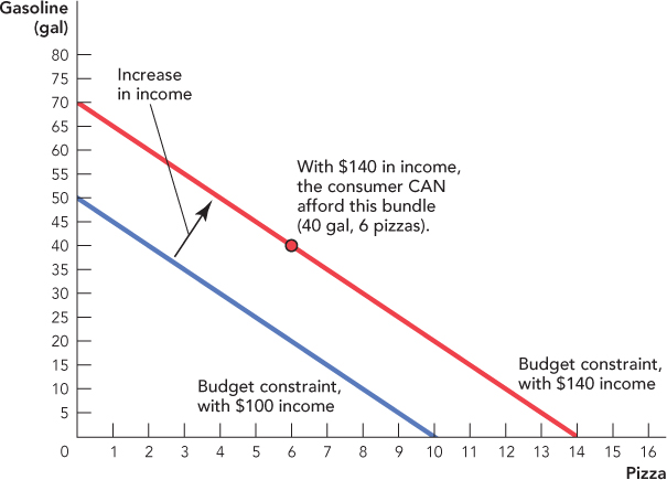
The budget constraint depends on the consumer’s income and also on the prices of gasoline and pizza. Let’s look at income first. Imagine, for example, that the consumer had $140 of income. Now the consumer could purchase any of the consumption bundles shown in Figure 25.5.

Notice that with $140 in income, the consumer can now afford the red consumption bundle (40 gallons of gasoline, 6 pizzas) that he could not afford with $100 income. More generally, an increase in income pushes the budget constraint outward, parallel to the old budget constraint.
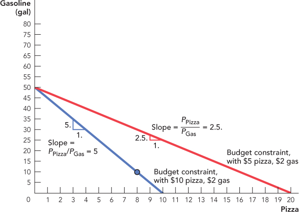
Now let’s look at how changes in prices affect the budget constraint. Assume that the consumer has $100 in income and the price of gasoline is $2 per gallon, but now there is a sale on pizzas so the price falls to $5 per pizza. If the consumer spends all of his money on gasoline, he can still purchase 50 gallons of gasoline and 0 pizzas so the point on the vertical axis remains the same. If he spends all his money on pizza, however, he can now afford 20 pizzas. Thus, as shown in Figure 25.6, a fall in the price of pizzas rotates the budget constraint outward along the horizontal axis.

 .
.471
CHECK YOURSELF
Question 25.1
 Draw a consumer’s budget constraint when the consumer has an income of $100, PGas = $2, and PPizza = $10. Now draw the new budget constraint when income = $80.
Question 25.2
 Draw a consumer’s budget constraint when the consumer has an income of $100, PGas = $2, and PPizza = $10. Now draw the new budget constraint when PGas = $4.
Question 25.3
 In 1970, the price of pizza is $2.50 and the price of a gallon of gas is $0.50. In 2010, the price of pizza is $10 and the price of a gallon of gas is $2. Has the relative price of pizza changed?
As you might expect from the figure, the slope of the budget constraint is closely related to the prices of pizza and gasoline. The slope of the budget constraint, the rise/run, tells us the trade-off between gasoline and pizza, that is, how many gallons of gasoline the consumer can afford if he buys 1 fewer pizza. When the price of a pizza is $10 and the price of a gallon of gas is $2, the consumer can afford 5 more gallons of gasoline when he purchases 1 fewer pizza, so the slope of the budget constraint is  . The slope of the budget constraint is also called the relative price. In this case, the relative price of pizza to gas is 5. To be precise, the slope of the budget constraint is –5, which reflects the fact that to get more gasoline, the consumer must purchase fewer pizzas, but economists often drop the negative sign for convenience (mathematicians, however, would be horrified at this practice).
When the price of pizza falls to $5 per pizza, the consumer can afford 2.5 additional gallons of gasoline when he purchases 1 fewer pizza, so the slope of the budget constraint falls to  . We can now draw a consumer’s budget constraint for any income and set of prices. We know that the consumer will choose a consumption bundle somewhere along the budget constraint, but to say more about the exact consumption bundle, we need to say more about preferences.
472