We have now developed the key tools that we need to better understand consumer and worker choice. Let’s begin with some applications of income and substitution effects.

478

Have you ever bought a concert or movie ticket and then lost it? When should you buy another ticket? If you lost your ticket, you probably feel foolish or angry. Many of us react emotionally in a situation like this, and perhaps we decide that fate is against us and that we weren’t really meant to see the concert or movie anyway. The better course of action, however, can be determined by some cooler thinking and a little economics.

Let’s say you lose a movie ticket on which you spent $10. What is the price if you wish to buy another ticket? It’s still $10. You are still comparing the movie against other uses for the $10. In terms of the substitution effect, the price hasn’t changed so there should be no change in your assessment. Either the movie is worth giving up $10 worth of other goods or it is not.

What about the income effect? Well, you’re out the $10 and thus you are poorer. That’s a fairly small negative income effect. If you’re really poor, though, it might induce you to make fewer purchases, including movie ticket purchases. But for most people, the income effect should be very small, so small that it can be safely ignored. Thus, if the ticket cost $10, you should buy another ticket.

Alternatively, let’s say you lose a Lady Gaga concert ticket, which cost you $200 on eBay. There is still no change in the price, at least assuming that the price on eBay hasn’t changed, so the logic of substitution still says buy another ticket. But now the negative income effect is larger than in the case of the movie ticket. It shouldn’t bother a well-off person, but some of you will feel noticeably poorer and you may wish to reconsider buying another concert ticket for $200.

The motto of the story: If you lose cheap tickets, replace them for sure. If you lose expensive tickets, you need to compare the income effect with the substitution effect. For a sufficiently wealthy person, even the loss of an expensive concert ticket shouldn’t create a very big income effect. Poorer people may wish to think twice.

Costco, one of the largest retailers in the world, offers low prices on many consumer goods. But to shop at Costco, you have to join the Costco “club” and pay a yearly membership fee. How much should Costco charge for membership?

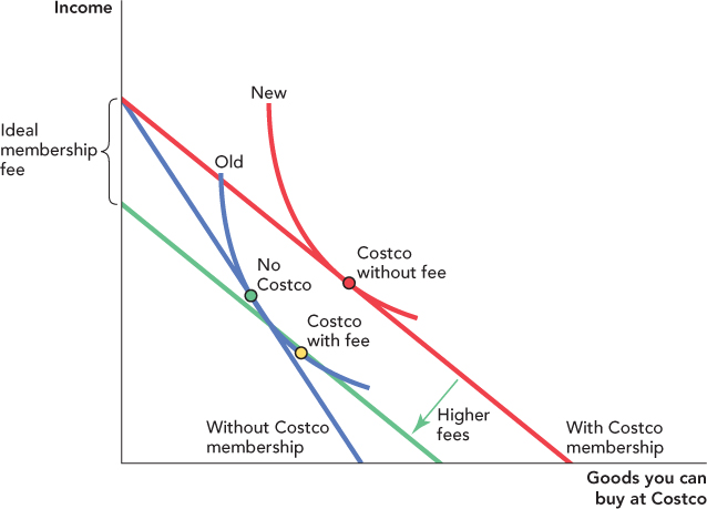
To answer this question, let’s create a budget constraint and indifference curve diagram with income on the vertical axis and goods you can buy at Costco on the horizontal axis. Without Costco membership, the consumer faces the blue budget constraint in Figure 25.12, labeled “Without Costco Membership,” and consumes the No Costco bundle. Costco members pay lower prices, so if there were no membership fee, Costco members would face the red budget constraint, labeled “With Costco membership,” and consume the “Costco without fee” bundle.

Costco, however, wants to charge as high a membership fee as possible. How much can the retailer charge? The membership fee is equivalent to a decrease in the consumer’s income, so another way of asking this question is to ask how much can we decrease the consumer’s income and still leave the consumer at least as well-off with Costco membership as without it? If we shift the green budget line, which reflects the lower prices at Costco, back toward the origin, we can shift the line until it is tangent to the old indifference curve at the point labeled “Costco with fee.” At “Costco with fee,” the consumer is indifferent between joining Costco, paying the fee, and enjoying the lower prices, and not joining Costco, saving on the fee, but paying higher prices. Since income on the vertical axis, we can easily read the ideal membership fee off the graph.

479

Costco charges $50 for membership. This may not seem like a lot, but in 2010 membership fees earned Costco revenues of $1.7 billion dollars, which exceeded its profits of $1.3 billion. Costco, therefore, is very concerned with setting the ideal membership fee.

In Chapter 18, we discussed how a worker’s labor supply curve can be backward-bending; that is, a decrease in the wage could cause a worker to work more. At first, this might seem surprising. Why would a worker work more hours when the payoff to working is going down? To see the intuition, imagine a janitor, perhaps an immigrant from a developing country, whose wage falls. The janitor may choose to work more hours in response to the lower wage, because at a lower wage, he needs to work more hours to make enough money to put his children through college. Similarly, when the Beatles were young and unknown, they were paid low wages but they played 4 to 5 sets a day, 7 days a week in German strip clubs, just to make ends meet. As their fame grew, so did their wages and the Beatles responded by playing fewer hours. Eventually, they stopped touring altogether, and a few years after that, they split up completely.

480

More generally, remember that a lower wage has two effects: the substitution effect and the income effect. When the wage decreases, that’s the same as a decrease in the price of leisure so the substitution effect says you should “buy” more leisure by working fewer hours. When the wage decreases, however, that also makes you poorer. The income effect says that when your income falls, you should buy fewer (normal) goods including leisure.

Notice that the substitution and income effects work in opposite directions in this case. If the substitution effect dominates, the worker works fewer hours when the wage rate falls. If the income effect dominates, the worker works more hours when the wage rate falls.

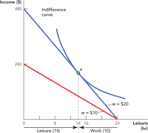
In Figure 25.13, we explain the basics of the income–leisure model of labor supply. We put income on the vertical axis and leisure on the horizontal axis. We will think about daily labor supply so the maximum number of hours of leisure is 24. Imagine that the wage is $20 an hour. If the worker chooses 24 hours of leisure (0 hours of work), she earns $0. If the worker chooses 0 hours of leisure (24 hours of work), she earns $480 a day. The budget constraint labeled w = $20, therefore, shows all the income–leisure possibilities open to the worker when the wage is $20 an hour. As usual, the optimum is found where the budget constraint is tangent to the indifference curve. At point a, the worker chooses 14 hours of leisure (10 hours of work).

Suppose the wage is cut to $10 an hour. If the worker chooses 24 hours of leisure, she still earns $0, but if the worker chooses 0 hours of leisure (24 hours of work), her take-home pay falls to $240. The budget constraint labeled w = $10, therefore, shows all the income–leisure possibilities open to the worker when the wage is $10 an hour. The worker will choose a new point (not shown) on the new budget constraint.

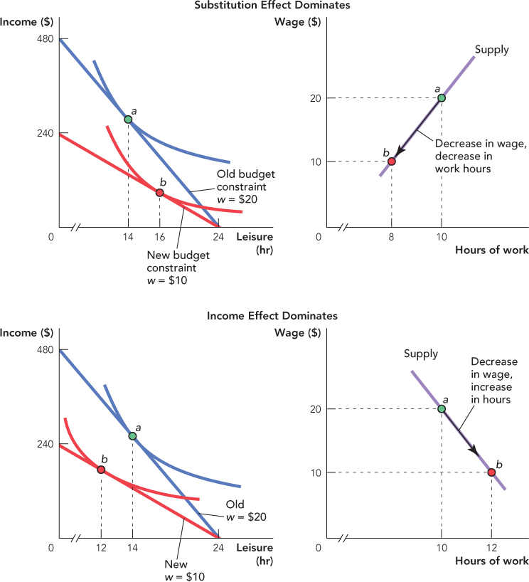
In Figure 25.14, we use this model to show how a decrease in the wage can decrease or increase labor supply. In the top left panel, the worker chooses 14 hours of leisure (10 hours of work) when the wage is $20 an hour. A decrease in the wage causes the worker to increase leisure to 16 hours (8 hours of work). We haven’t drawn the substitution and income effects in the diagram (we leave that as an exercise), but since the total effect of the decrease in wages is a decrease in labor supply, we know that in this case the substitution effect dominates. The top right panel translates the same information into a labor supply diagram.

481

In the bottom left panel, the worker chooses 14 hours of leisure (10 hours of work) when the wage is $20 an hour. A decrease in the wage causes the worker to decrease leisure to 12 hours (12 hours of work). Since the total effect of the decrease in wage is an increase in labor supply, we know that in this case the income effect dominates. The bottom right panel shows that over this wage range, the worker has a backward-bending labor supply curve.

482

Let’s use the income–leisure model to examine the labor supply effects of welfare programs. The traditional model of welfare works like a guaranteed minimum income under which the government subsidizes or “tops up” the income of any worker who earns less than the guaranteed amount. For example, suppose the guaranteed minimum income for an individual is $10,000 a year; in that case, an individual with yearly earnings of $6,000 would receive $4,000 in welfare payments.

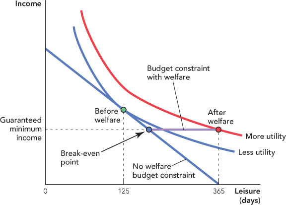
The economics of this program are shown in Figure 25.15. We use the same setup as before, only now we measure leisure and work on a yearly basis in days rather than on a daily basis in hours. Before the welfare program, the worker faces the No welfare budget constraint and chooses 125 days of leisure (240 days of work.) The guaranteed minimum income expands the worker’s opportunities. In particular, the worker now has the option of taking the guaranteed income and 365 days of leisure. The worker pictured earns more utility by taking the option of the guaranteed minimum income and the 365 days of leisure. Not every worker will take the guaranteed minimum income, but every worker who does take the option will reduce work effort.

We can explain why the guaranteed minimum income reduces work effort in a second way. Consider again how a guaranteed minimum income of $10,000 works. If a worker earns $2,000, she receives $8,000 in welfare for a total of $10,000. If a worker earns $4,000, she receives $6,000 in welfare for a total of $10,000. If a worker earns $7,000, she receives $3,000 in welfare for a total of $10,000. Do you see a pattern? Under the guaranteed minimum income, for every $1 in income that the worker earns, the government subtracts $1 in welfare so the worker’s take-home pay doesn’t change. Thus, under the guaranteed minimum income, a worker faces a 100% tax rate until he is earning more than $10,000 a year (the break-even point). Thus, under a guaranteed minimum income, many workers will choose to work 0 hours. How many hours would you work if you faced a 100% marginal tax rate?

483

On the one hand, most people feel that a welfare program is necessary to help those in need. On the other, we don’t want to discourage work effort. Even a low-paying job, for example, may lead to a higher-paying job in the future. The trade-off between ethics and the disincentive effects of welfare programs have bedeviled policymakers for decades. In fact, for hundreds of years, economists like Adam Smith and John Stuart Mill have worried about this problem.1

Several resolutions to this trade-off have been suggested, none of which is perfect. We will mention two briefly. One possibility is to focus on the 100% tax rate faced by people on welfare. Instead of reducing the welfare payment by $1 for every $1 of earnings, how about reducing payments by, say, $0.50 for every dollar of earnings? This is called a negative income tax (NIT) program. Under a negative income tax, for example, a worker who works 0 hours would receive $10,000 in welfare for a total of $10,000. But a worker who earned $4,000 would receive $8,000 in welfare (not $6,000 as before) for a total of $12,000. In this way, some of the incentives to work are restored for those receiving welfare.

Unfortunately—precisely because the program is more generous—the negative income can encourage more people to reduce labor supply at least somewhat and to take at least some welfare, even if they are able to work. Under the traditional guaranteed income program, for example, a worker who was earning, say, $14,000 a year might refuse the option of $10,000 a year and 365 days of leisure, but under a negative income tax, that same individual might be happy to accept $12,000 a year with 200 days of leisure.

Even though the negative income tax can encourage some people to partially reduce their hours of work, it encourages everyone to have at least some kind of job. If having a job, even a part-time job, is what matters for gaining experience, learning skills, moving up the work ladder, and so forth, then the NIT may work acceptably well.

Another approach is to limit how much welfare a person can accept or put various requirements on welfare recipients. If a person knows in advance that welfare is available only for a limited time, for example, he or she will treat welfare as more of an insurance program to be used only in bad times rather than as a guaranteed minimum income to be used as an alternative to work.

In practice, the United States has pursued both of these approaches to various degrees. The Earned Income Tax Credit (EITC), for example, supplements the wages of low-wage workers. For instance, depending on your income and other factors, if you earn $100 at work, the government tops it off, through the tax system, to make it worth $120. Unlike a negative income tax, the EITC is available only to workers. The EITC, however, helps offset the incentive to quit work, as contained in some of the other welfare programs, and makes the total package more like a negative income tax. From another direction, the Personal Responsibility and Work Opportunity Reconciliation Act (PRWORA) of 1996 put limits on welfare. Under PRWORA, a person can receive only 5 years of welfare benefits over his or her lifetime, and after 2 years on welfare, recipients must work at least 30 hours a week.

Both of these programs appear to have been relatively successful at encouraging welfare recipients to enter the job force. Analyzing the incentive and disincentive effects of welfare programs continues to be an active area of research for economists.

484