Nominal vs. Real GDP
The rate of growth just calculated did not adjust for price changes and is called the “nominal growth rate.” The alternative concept is the growth rate of real GDP and here is the background for understanding that distinction.
Nominal variables, such as nominal GDP, have not been adjusted for changes in prices.
Nominal GDP is calculated using prices at the time of sale. Thus, GDP in 2013 is calculated using 2013 prices and GDP in 2000 is calculated using 2000 prices. If we want to compare GDP over substantial periods, using nominal GDP creates a problem. GDP in 2013, for example, was $16.8 trillion and GDP in 2000 was $10.3 trillion. Should we celebrate this roughly 63% increase in GDP 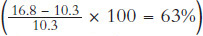 ? Not so fast! Before we celebrate, we would like to know whether the increase was due mostly to greater production—more cars and more chickens—or to increases in prices between 2000 and 2013.
Economists usually are more interested in increases in production than increases in prices because only increases in production are true increases in the standard of living. But how can we measure increases in production while controlling for increases in prices? Here is what we know so far:
2013 nominal GDP = 2013 prices × 2013 quantities = $16.8 trillion
2000 nominal GDP = 2000 prices × 2000 quantities = $110.3 trillion
Can you see how to compare the increase in production from 2000 to 2013? Suppose we calculate GDP in 2000 using 2013 prices instead of 2000 prices. The U.S. Bureau of Economic Analysis does just this and finds the following:
2013 GDP in 2013 dollars = 2013 prices × 2013 quantities = $16.8 trillion
2000 GDP in 2013 dollars = 2013 prices × 2000 quantities = $13.8 trillion
SEARCH ENGINE
You can find data on U.S. real and nominal (“current dollar”) GDP from the Bureau of Economic Analysis, http://www.bea.gov/national/.
What this tells us is that if prices in 2000 were the same as in 2013, then GDP in 2000 would have been measured as $13.8 trillion. Economists also say that 2000 GDP in 2013 dollars is real GDP in 2013 dollars. Since 2013 GDP is already in 2013 dollars, it’s also real GDP in 2013 dollars.
Now that we have real GDP in 2000 and real GDP in 2013, we can find the increase in real GDP. Between 2000 and 2013, the increase in real GDP was 21.7% 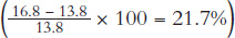 . Thus in 2013 the economy produced 21.7% more stuff, goods, and services than in 2000. That’s not a great performance and quite a bit less than the value we calculated earlier—63%—because prices also increased during this period.
If we want to compare GDP over time, we should always compare real GDP, that is, GDP calculated using the same prices in all years. Interestingly, it doesn’t matter much what prices we use to calculate real GDP, so long as we use the same prices in all years.
Real GDP calculations become trickier, the longer the period we compare. In 1925, for example, what was the price of a computer? Economists and statisticians involved in calculating real GDP must worry about the value of new goods and changes in the quality of old goods. The more years that pass, the more difficult it is to determine how to adjust for those quality changes.
Real variables, such as real GDP, have been adjusted for changes in prices by using the same set of prices in all time periods.
The real versus nominal distinction is an important one in economics and it will recur throughout this book. A real variable is one that corrects for inflation, namely a general increase in prices over time. In later chapters, we will discuss the real price of housing, real wages, and the real interest rate and we will show in more detail how to convert nominal data into real data.
The GDP Deflator
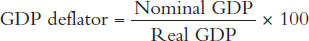
The GDP Deflator is a price index that can be used to measure inflation. We will be discussing price indexes and inflation at greater length in Chapter 31. The GDP Deflator, however, is very easy to calculate once we know nominal and real GDP for a given year. The GDP deflator is simply the ratio of nominal to real GDP (multiplied by 100).
For example, let’s calculate the GDP deflator for 2013. We can easily find 2013 nominal GDP and 2013 real GDP (using 2009 dollars) from the U.S. Bureau of Economic Analysis. Here are the numbers:
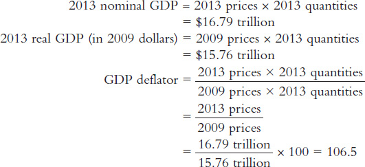
To see why the GDP deflator can be used to measure inflation, notice that the deflator is a ratio of prices. What the deflator tells us is that 2013 prices were about 6.5% higher (106.5 − 100) than 2009 prices.
Real GDP Growth
If pressed to choose a single indicator of current economic performance, most economists would probably choose real GDP growth. Figure 26.3 shows the annual percentage changes in real GDP for the United States from 1948 to 2013. U.S. real GDP growth was high during the 1960s, but rising inflation and the 1973 and 1979 oil price shocks lowered growth in the 1970s and early 1980s. Growth was more solid after the 1982 recession until the mid-2000s but still somewhat lower than in the 1960s. The severe recession of 2009 and slow recovery since then is also evident in the figure. Note that the long-term (since 1948) average growth of real U.S. GDP has been about 3.25% per year. You can use these figures as benchmarks to gauge current growth rates.
FIGURE 26.3

Source: Bureau of Economic Analysis.
Real GDP Growth per Capita
Growth in real GDP per capita is usually the best reflection of changing living standards. Growth in real GDP typically gives the same broad idea of how economic conditions are changing as growth in real GDP per capita, but there can be big differences for countries with rapidly growing populations. For instance, between 1993 and 2003, Guatemala experienced real GDP growth of about 3.6% a year. That might sound good but over that same period population grew at 2.8% a year, so real GDP per capita in Guatemala grew at just 0.8% a year. In comparison, real GDP per capita in the United States typically grows by about 2.1% a year. Thus, not only is the United States richer than Guatemala, people in the United States are getting richer faster.
Figure 26.4 shows average annual growth rates of real GDP per capita across the globe for a long-run period. The green-colored nations experienced average growth rates of greater than 2% over the entire period. Taiwan, for example, averaged 6% growth of real GDP per capita per year. On the other end of the spectrum, the nations in dark red were growth disasters: They saw declines in GDP per capita over this period.
FIGURE 26.4

CHECK YOURSELF
Question 26.5
 Name a country with a high GDP but a low GDP per capita.
Question 26.6
Name a country with a low GDP but a high GDP per capita.
Question 26.7
Why do we often convert nominal variables into real variables?
Nigeria is a tragic example of a growth disaster. In 1960, when Nigeria gained its independence from Great Britain, vast deposits of oil were discovered and the future looked bright. But a vicious civil war, dictatorship, and massive corruption meant that the oil wealth disappeared in arms purchases and secret Swiss bank accounts. Incredibly for an economy in the modern era, real GDP per capita in Nigeria was a little bit lower in 2000 than it had been in 1960.
Although it seems shocking that a country could be no richer in 2000 than in 1960, it’s important to remember that throughout most of human history, a failure to grow is normal. In the next chapter, we will begin to explain not only why some nations are poor but the truly mysterious question: Why are any nations rich?