Let’s stay with the Solow model a little longer and look at investment rates and conditional convergence.

What happens in the Solow model if 7, the fraction of output that is saved and invested, increases? It is simple: A greater investment rate means more capital, which means more output. An increase in the investment rate therefore increases a country’s steady-state level of GDP. The result just shows that investment increases the number of “tractors” per worker, which raises GDP per worker.

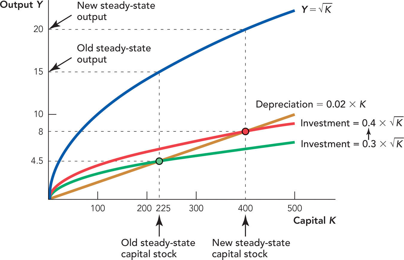
In Figure 28.7, we show this intuition in the graph by plotting two investment functions: , which means that 3 units of every 10 units of output are saved and invested (7 = 0.3, as it was in Figure 28.6), and also , which means that 4 units of every 10 units of output are saved and invested (γ = 0.4). Notice that when γ = 0.4 the new steady-state capital stock increases to K = 400 and output increases to 20.

152

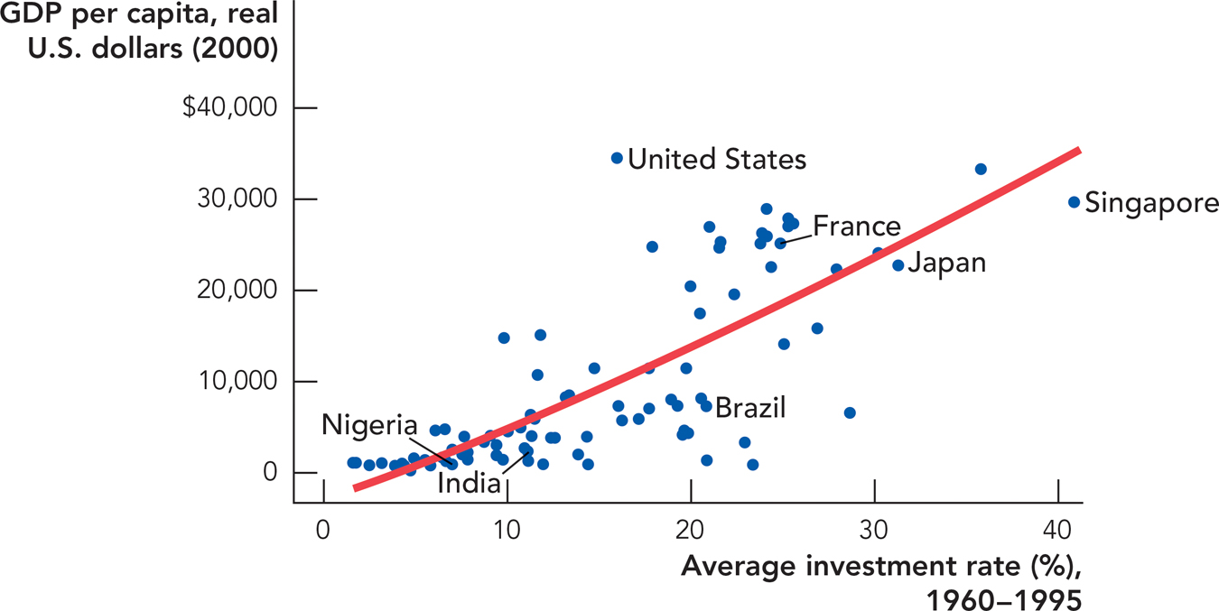
Thus, the Solow model predicts that countries with higher rates of investment will be wealthier. Is this prediction of the Solow model consistent with the evidence? Yes. Figure 28.8 shows that GDP per capita is higher in countries that have higher investment rates.

153

This makes intuitive sense. More savings mean that more capital goods can be produced and consumers can enjoy a higher standard of living. How wealthy would a country be if it spent all of its resources on partying?

The Solow model says that an increase in the investment rate will increase steady-state output. But in the Solow model, the iron logic of diminishing returns cannot be avoided. When the investment rate increases, we have Investment > Depreciation so the capital stock increases and the economy grows. But as more capital accumulates, the iron logic sets in and the economy eventually slows until at the new steady state it stops growing once again. So the level of the capital stock determines the output level but not its growth rate, at least not in the very long run.

For further confirmation of this idea, recall the growth miracle of South Korea from the last chapter. In 1950, South Korea was poorer than Nigeria, while today it is richer than some European nations. The evidence on South Korea’s growth is consistent with the Solow model. In the 1950s, the investment rate in South Korea was less than 10% of GDP, but the rate more than doubled in the 1970s and increased to more than 35% by the 1990s. Higher investment rates helped to increase South Korea’s GDP, as the country opened many factories and exported cars and electronics to the rest of the world. As South Korea has caught up to Western levels of GDP, however, its growth rate has slowed.

Of course, we should remember that investment rates are themselves caused by other factors such as incentives and institutions. No one wants to invest in an economy, for example, where their investments may be expropriated. One of the reasons the investment rate in South Korea increased is that capitalists believed their investments would be protected.

In this chapter, we have referred to γ as the rate of savings and investment, implicitly assuming that savings equals investment. But savings must be efficiently collected and then transformed into investment. The Soviet Union had a high rate of saving but its savings were not invested well, and thus its effective investment rate was very low. In other words, a country that invests its savings poorly is like a country that doesn’t invest much at all. A country could also have a low rate of saving but a high rate of investment if it imported savings from other countries. The next chapter will discuss in more detail how financial intermediaries efficiently collect savings, often from around the world, and then transform those savings into productive investments.

The Solow model also predicts that a country will grow more rapidly the farther its capital stock is below its steady-state value. To understand this result, remember that when the capital stock is below its steady-state value, investment will exceed depreciation. In other words, the capital stock will grow. Now look again at Figure 28.1—when the capital stock is low, it has a very high marginal product. Thus, when a country’s capital stock is below its steady-state value, the country will grow rapidly as it invests in capital that has a high marginal product. That’s just restating our tractor parable. The tractor is most valuable on the farm that doesn’t already have a tractor, as opposed to the farm that is already working with 13 tractors. (A more detailed explanation of this point can be found in the appendix to this chapter.)

154

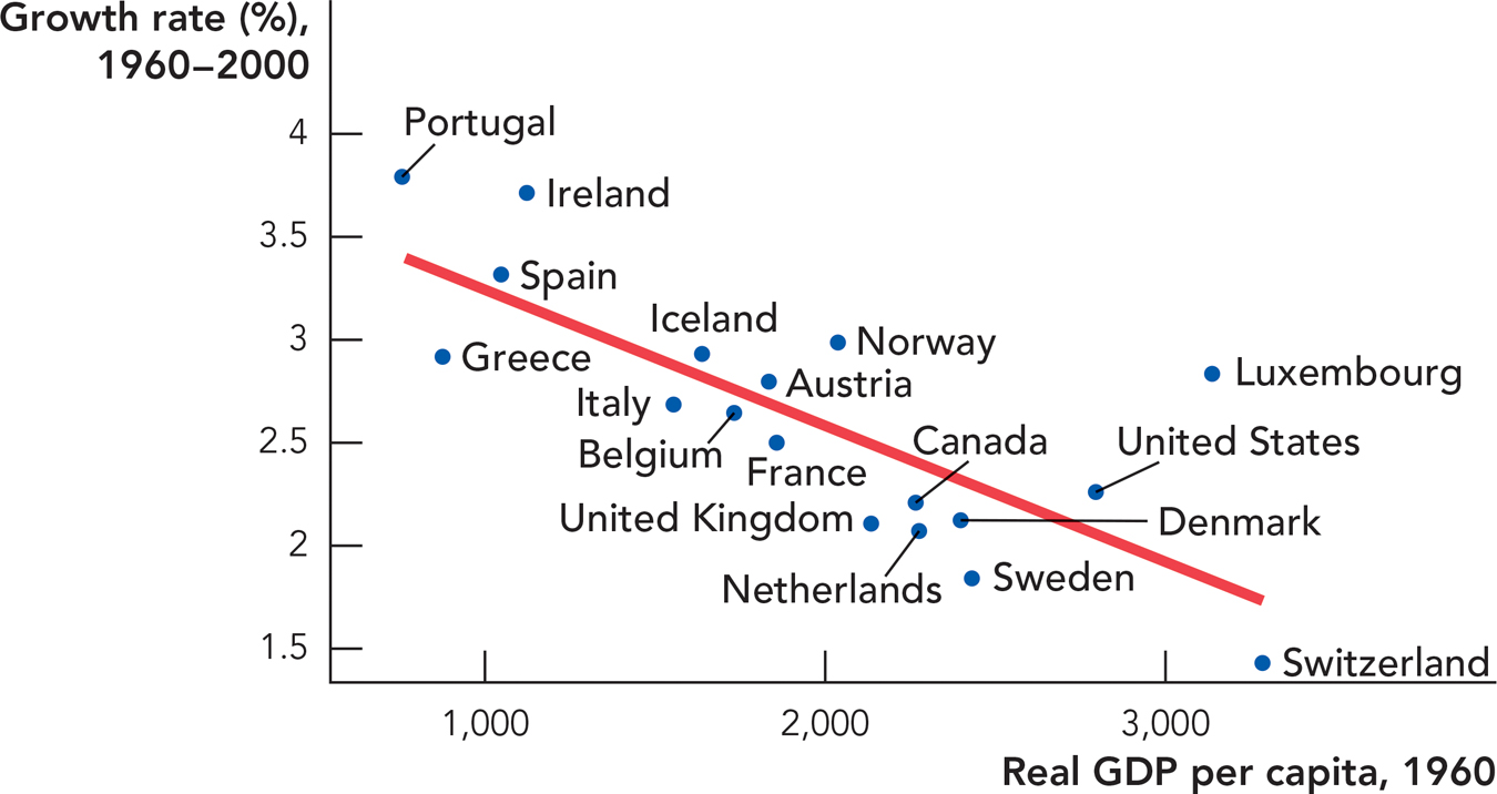
We already used this result to explain why China is growing rapidly and why Germany and Japan grew rapidly after World War II. More generally, the Solow model predicts that if two countries have the same steady-state level of output, the country that is poorer today will catch up because it will grow faster. We don’t know for certain which countries have the same steady-state level of output, but we might guess, for example, that countries with similar institutions and history have similar steady states. Figure 28.9 tests this prediction using data from 18 of the 20 founding members of the OECD (Organisation for Economic Co-operation and Development).1 The average annual growth rate between 1960 and 2000 is on the vertical axis, and real per capita GDP in 1960 is on the horizontal axis. The data clearly show that among the OECD countries the poorer countries grew faster. You can see that lower income in 1960 is associated with higher growth between 1960 and 2000.

Since the poorer countries grow faster, they eventually catch up to the richer countries. Thus, over time the OECD countries have converged to a similar level of GDP per capita. We say that the model and the data exhibit conditional convergence because we only see convergence among countries that plausibly have similar steady-state levels of output. As we know from Chapter 27, we do not observe convergence among all countries—the existence of growth disasters such as Nigeria means that some countries are diverging from the rest of the world rather than catching up.