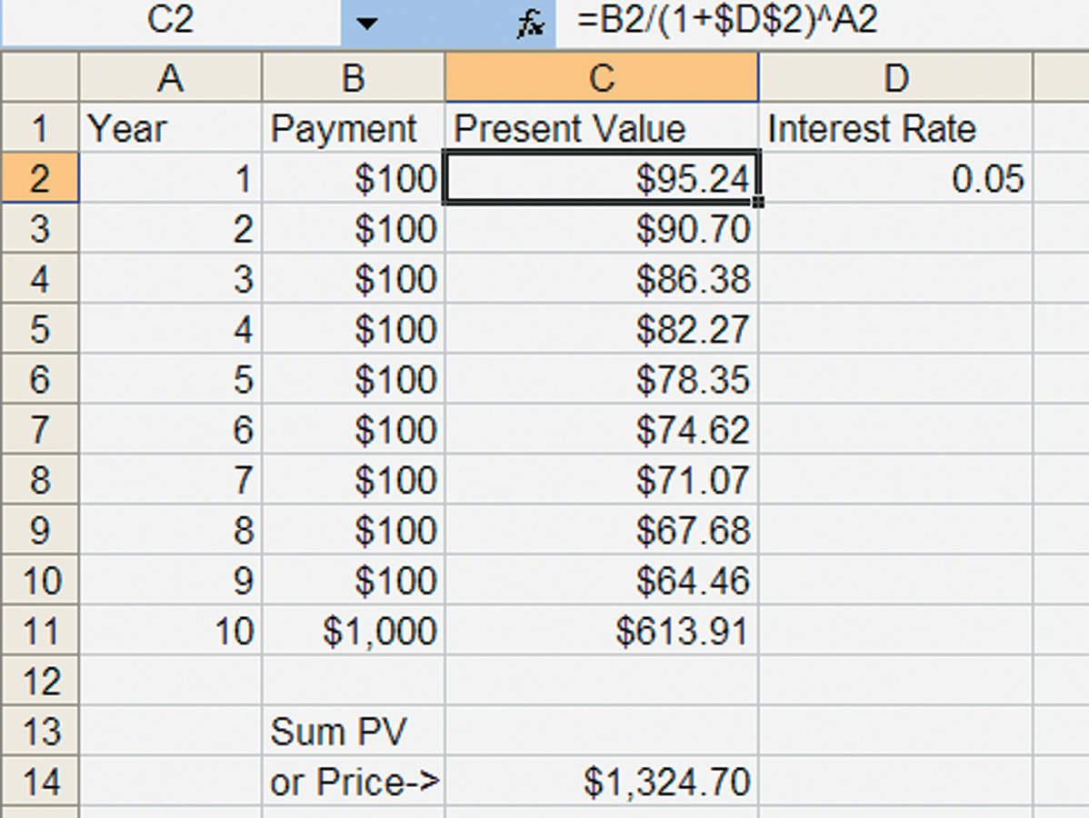
We can calculate the price of bonds like this using a spreadsheet. Figure A29.1 shows a bond that pays $100 in each of the first nine years and then in the 10th year it pays $1,000. The present value of each payment is calculated in Column C. Note that the formula in cell C2,“=B2/(1+$D$2)^A2”, is equivalent to . Copying this formula for the nine other payments gives us a column of present values, which we sum up in cell C14,”=SUM(C2:C11)”, to find the price of the bond, $1,324.70.

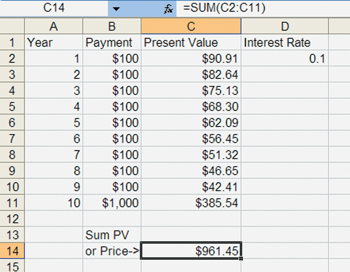
You can easily vary the interest rate to see what happens to the price of the bond. If the interest rate rises to 10%, for example, we have the result in Figure A29.2 below.

206

And thus, the price of the bond falls to $961.45. Note once again that a higher interest rate means a lower price for the bond. It’s also interesting to see that a higher interest rate has a small effect on payments that come soon (compare the PV of the first payment in Figure A29.1 and Figure A29.2), but a very large effect on payments far into the future (compare the PV of the final payment in the two scenarios).

One final point of importance. Bond pricing might seem to be far away from your interests, but the techniques in this appendix can be used to price and understand any kind of asset that has a payment stream over time. A mortgage, for example, is very similar to a bond except instead of receiving bond payments, you will typically be sending mortgage payments. If you want to compare two different mortgages, for example, a 20-year mortgage and a 30-year mortgage where the mortgages have different interest rates, you will want to compute the present value of each mortgage to find the one with the lowest PV. Online mortgage calculators help you to do this. What those calculators do is compute present values using the same types of techniques as found in this appendix.

* In principle, it is possible for the supply curve for savings to be negatively sloped. For instance, if an individual wanted exactly $100 in one year’s time, then at an interest rate of 10%, he or she would need to save $90.91, but at an interest rate of 20%, he or she would need to save only $83.33. Thus, an increase in the interest rate could reduce savings. The evidence, however, indicates that individual savings rates typically respond positively to higher interest rates. In addition, higher U.S. interest rates also encourage lenders in other countries to move some of their savings to U.S. markets. Both forces mean that the supply curve for savings is upwardly sloped in most circumstances.