Let’s take a closer look at real shocks. Real shocks are rapid changes in economic conditions that increase or diminish the productivity of capital and labor, which in turn influences GDP and employment. To understand shocks and to see why they matter, we start with poorer economies, where shocks are easier to see and understand. Later in the chapter, we move to how shocks can create problems for the U.S. and other developed economies.

There are several billion farmers in the world and for many countries agriculture remains the single largest contributor to GDP. How much a farm produces depends on the quantity and quality of the inputs of capital and labor, but agricultural output also depends on the weather. When the weather fluctuates, so does output and therefore so does GDP, especially in agricultural economies.

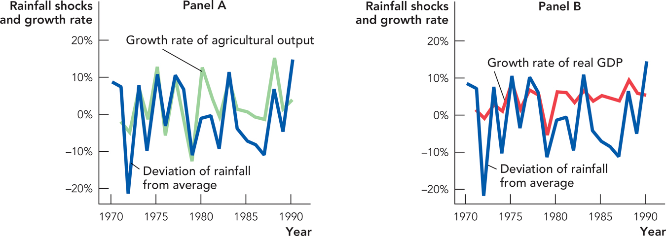
Figure 32.8 shows how shocks to the weather influence India’s agricultural output and GDP. The blue line is the percentage deviation in India’s yearly rainfall from the average (from 1970 to 1990). Above-average rainfall is good for the crops so in 1975, for example, rainfall was 10.8% above average, and in the left-hand panel, we see that agricultural output in that year grew by a bountiful 12.8%. In 1979, however, much of India had a drought. Rainfall was 11% below average and agricultural output fell by nearly 13%, compared to the year before.

281

When India’s agricultural output falls, so does India’s GDP. It is not just that agriculture contributes to GDP directly but, if farmers struggle, many other sectors of the Indian economy suffer as well. For instance, the demand for tractors will go down and farmers will buy fewer items for their own consumption. Thus, the shock spreads to other sectors of the economy.

Agriculture has been the largest contributor to India’s GDP, so the shocks to agricultural output caused by the weather have had a big impact on GDP growth. In Panel B of Figure 32.8, the red line shows the growth rate of India’s GDP. As expected, GDP boomed in 1975, growing by nearly 10%, and busted in 1979 with a decline of 5.2%. Note that the booms and busts in GDP are not as strong as the booms and busts in agricultural output because other sectors, less influenced by the weather, also contribute to GDP.

By the way, take a close look at Panel B of Figure 32.8. Does it seem to you that shocks to rainfall have become less important to India’s GDP since 1980? If so, you are probably correct. Agriculture contributed 40% of India’s GDP in 1970, but because the Indian economy has grown and diversified, it contributed only 20% of India’s GDP in 1990. Therefore, shocks to the weather are becoming less economically important in India over time. In the United States, agriculture contributes less than 1% to GDP, so yearly variations in the weather don’t have much of an effect on GDP. Other shocks, however, can rock the U.S. economy.

In an economy with a large manufacturing sector, a reduction in the oil supply is like a reduction in rainfall in an agricultural economy. Oil and machines are complementary, which means they work together, along with labor, to produce output. Thus, when the oil supply is reduced, capital and labor become less productive. Oil greases the wheels of industry, sometimes literally, and with less oil the wheels do not turn as well.

The first oil shock came in late 1973, when many of the oil-producing nations under the guise of OPEC (Organization of the Petroleum Exporting Countries) reduced the global oil supply to protest America’s support of Israel in the Middle East. The result was that the price of oil more than tripled in just two years. This became a significant problem for the American economy.

The higher price of oil, for instance, also meant a much higher price for gasoline (oil is one input into gasoline). Higher gas prices reduced the demand for larger cars and increased the demand for smaller cars. The U.S. auto industry was specialized in the production of larger cars and had a difficult time adjusting. Factories cannot simply be switched from the production of one type of car to another—much of the physical capital in an auto factory is specialized. A machine that is used to bend steel is no longer useful when production switches to lightweight, fuel-saving plastic composites. Workers are specialized, too, in both knowledge and location. Thus, the oil shock meant that many auto plants producing larger cars shut down or were used at less than full capacity. Similarly, autoworkers became unemployed and many had to learn new skills, and often they had to move to new jobs.

Not every part of the American economy was harmed. The demand for smaller cars increased, for example, but the U.S. auto industry could not immediately meet that demand. It can take a decade to design and build a new car, so it took considerable time for capital and labor to reallocate to the production of smaller American cars. In the meantime, output and employment in the auto industry fell. Similarly, over time, the city of Houston (which services much of the American oil industry) became populated with many former residents of Detroit (which made large American cars), but the transition was costly and disruptive.

282

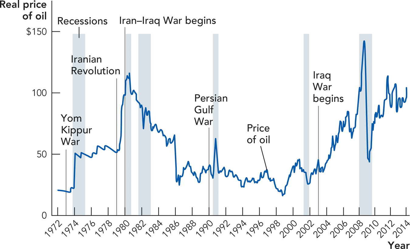
Since oil is an important input in many sectors of the economy, high oil prices—or oil shocks—hurt many American industries. Thus, sharp increases in the price of oil can disrupt the economy as a whole. Figure 32.9 shows the price of oil and the last six U.S. recessions. In each case, there was a large increase in the price of oil just prior to or coincident with the onset of recession (oil prices were still very high during the 1981-1982 recession, which was almost a continuation of the 1980 recession). The pattern is especially clear with the 1974, 1980, and 1991 recessions in the graph. In these cases, the onset of a war reduced the supply of oil, driving up the price unexpectedly. Unexpected shocks are the most costly to deal with.

It’s fairly easy to see the impact on the economy of a large increase in the price of oil but it’s harder to eyeball the effect of smaller shocks. Careful statistical analysis, however, can disentangle the effect of oil shocks from the many other shocks that keep on hitting the economy. In Figure 32.10, we show how the economy responds to an unexpected and permanent increase in the price of oil of 10%.

Starting from the normal or trend rate of growth (which is fixed at the zero point on the vertical axis of the graph), Figure 32.10 shows that a 10% increase in the price of oil slows the economy down gradually, with the biggest slowdown occurring about 5 quarters (a little over a year) after the onset of the increase in price. After 5 quarters, the growth rate begins to pick up again quite quickly, and after 10 quarters (two and a half years), the economy has adjusted to the higher price and the growth rate returns to normal.

Thus, a 10% increase in the price of oil lowers the GDP growth rate, from what it would have been without the price increase, for just over two years. The total effect on GDP is a decrease of about 1.4%. In other words, if the price of oil had not increased, real GDP would have been about 1.4% higher.

283

Oil and rainfall shocks are only two among many shocks that might hit an economy. Other possible shocks are wars, terrorist attacks, major new regulations, tax rate changes, mass strikes, and new technologies such as the Internet. Most generally, economies are continually hit by many small shocks. Some of the shocks are good, like a productive new technology, and some are bad, like a drought. In a typical year, the good shocks outweigh the bad and the economy grows. People build on previous knowledge and most of the time they are able to do better and produce a bit more than in previous years. In a bad year, however, an economy may be hit with a big shock, like an oil shock, or more small shocks are negative than positive and a recession results. It is a bit like playing poker. Every now and then you get a hand of cards that simply cannot be played well, no matter what else you do. Table 32.1 lists some major factors that shift the LRAS curve left (negative shock) or right (positive shock).

284

In addition to shocks, there are also forces that amplify and transmit shocks across sectors of the economy and through time. In the next chapter, we will take a closer look at amplification and transmission mechanisms and show how a shock to, for example, the agricultural sector can be amplified and transmitted to many other sectors of the economy in a way that can make the shock have bigger effects and last longer than might be expected from the size of the shock alone.