The Great Depression (1929-1940) was the most catastrophic economic event in the history of the United States. GDP plummeted by 30%, unemployment rates exceeded 20%, and the stock market fell to less than a third of its original value. America went from confidence to desperation. In fact, the Great Depression was a worldwide event, plaguing almost all the developed nations. In some cases, such as Germany, the economic downturn led to totalitarian regimes followed by war. The 1930s and 1940s were terrible years for the world and bad economic policy was partly at fault.

The Great Depression occurred in the United States as follows. In 1929, the stock market crashed, creating a mood of pessimism among the American public. In part, this stock market crash had been brought on by a tight monetary policy, aimed at limiting a stock market bubble. The fall in stock prices was a wealth shock that made many people feel poorer and so they limited their spending, causing to fall. This, combined with the initial monetary contraction, that is, a reduction in , reduced aggregate demand, shifting the AD curve inward to the left.

But that is only the beginning of the story. In 1930, depositors lost confidence in their banks and, as they withdrew their money, they created a wave of bank failures. These bank failures meant that people lost their money, again diminishing aggregate demand. Moreover, at the time there was no government deposit insurance so when the first banks failed, people became suspicious of other banks and rushed to withdraw their money even from banks that were otherwise sound. From 1930 to 1932, there were four waves of banking panics; by 1933, more than 40% of all American banks had failed.

The fear and uncertainty created by bank failures, rising unemployment rates, falling consumer confidence, and inconsistent policymaking in Washington also reduced investment spending. Between 1929 and 1933, for example, investment spending fell by nearly 75%. In many years, spending on new investment was not enough to replace the tools, machines, and buildings that had depreciated due to natural wear and tear. Astoundingly, the U.S. capital stock was lower in 1940 than it had been in 1930.1

Furthermore, in 1931, instead of increasing , the Federal Reserve allowed the money supply to contract even further. In the early 1930s, the U.S. money supply fell by about a third, the largest negative shock to aggregate demand in American history. At that time, the Fed should have been expanding the money supply to drive up output in an emergency situation and also to boost the reserves of failing banks (we analyze monetary policy further in Chapter 35). Instead, the Fed allowed the money supply to contract and a disaster ensued. Bad decision making caused an additional monetary contraction during 1937-1938, which led to yet another wave of economic distress. It made the Great Depression much longer than it needed to be.

Figure 32.16 shows the story in a diagram. In the late 1920s, the economy was growing at a rate of about 4% per year with no inflation. Starting in 1929, a series of brutal shocks to aggregate demand reduced , , and and by 1932 pushed real growth to a rate of -13% and inflation to -10% per year. Note that although drawn separately, all these shocks were interconnected, as previously discussed.

293

To make all these problems worse, the decrease in aggregate demand caused prices to fall (as shown in the figure) and that, in turn, raised the real value of debts. One feature of virtually all loans is that they are denominated in terms of dollars, and the debt is not adjusted for inflation or deflation. So if a person or company has borrowed $10,000 and the price level falls by 10% (as it did in some of the Depression’s worst years), the real, inflation-adjusted value of that debt burden is now 10% higher than before. That makes life more difficult for debtors, and many of them will not be able to meet their obligations and perhaps they will go bankrupt, disrupting the economy further. Furthermore, many debtors will spend less money, thereby decreasing aggregate demand even more than from the initial shocks. While the real income of creditor banks goes up for the same reason that the real value of the debt goes up, these banks don’t have such a high propensity to spend or invest as do the desperate debtors, and so, the transfer of wealth from debtors to creditors still means that aggregate demand goes down.

Thus, the Great Depression was due primarily to the great fall in aggregate demand. Real shocks, however, also played a role in the Great Depression and in the failure of the economy to recover more quickly from the great fall. Let’s take a look at how real factors contributed to the Great Depression.

We have already mentioned one real shock—the bank failures—and you can see why bank failures are a real shock by thinking back to Chapter 29 on financial intermediation. Bank failures reduced the money supply and spending (an aggregate demand shock), but they also reduced the efficiency of financial intermediation. As we discussed in Chapter 29, banks play a key role in bridging the gap between savers and investors, and as banks failed, this bridge collapsed. Some firms could rely on internally generated funds for investment, and large firms could turn to the stock and bond markets for new funds. But many small businesses relied on loans from local banks that understood these businesses, and thus many small firms were especially harmed by bank failures.

294

To sum up the causal chain of events: A fall in reduced aggregate demand, which led to bank failures, which led to a reduction in the productivity of financial intermediation, a real shock. As you would by now expect, the real shock reduced growth even further. One of the broader lessons of this episode—which is true more generally—is that shocks to AD and shocks to the LRAS curve are linked in most recessions. In some cases, the shock to AD creates a real shock, and in other cases, a real shock creates a shock to AD; for instance, the fear and uncertainty created by a real shock can reduce AD by inducing people to cut back on spending and investment.

Some economic policy mistakes during the Great Depression also impeded recovery. As we have already mentioned, the Federal Reserve failed to use its power over the money supply to increase aggregate demand. In addition, there were other policy failures. For example, the National Industrial Recovery Act (NIRA) and the Agricultural Adjustment Act (AAA), both of 1933, tried to combat falling prices not by increasing aggregate demand but by reducing supply. Under NIRA, businesses were encouraged not to invest in machinery (in order to keep labor demand high), and they were encouraged to raise prices by creating cartels. Under the AAA, the government paid farmers to kill millions of pigs and plow under cotton fields in order to increase prices. Neither of these policies is likely to have increased economic growth. The Supreme Court ruled in 1935 and 1936, respectively, that both laws were unconstitutional.

Most famously (but perhaps not most importantly) the Smoot-Hawley Tariff of 1930 raised tariffs (taxes) on tens of thousands of imported goods.2 In principle, a tariff, by taxing foreign goods, can boost demand for domestic goods, thereby increasing AD. (Notice from Table 32.2, our list of factors that can shift AD, that a decrease in imports can increase AD.) In reality, retaliations against the Smoot-Hawley Tariff by other countries created a spiraling decline in world trade. When other countries raised their tariffs, U.S. exports fell. Remember that a reduction in exports reduces aggregate demand. Unfortunately, the large decline in world trade meant that the net effect of the tariff was to reduce aggregate demand.

A second negative effect of the tariff occurred because a tariff is a negative productivity shock. We get the most output from our capital and labor when we specialize in fields in which we have a comparative advantage and then trade for the goods that we produce at a comparative disadvantage (see Chapter 2 for more on comparative advantage). A tariff pushes capital and labor into lower productivity sectors, thereby reducing total output. Another way of seeing this point is to recognize that a tariff has exactly the same effects as an increase in transportation costs. Therefore, a tariff is like a negative productivity shock to the shipping industry, which ripples out to all the other industries dependent on shipping.

295

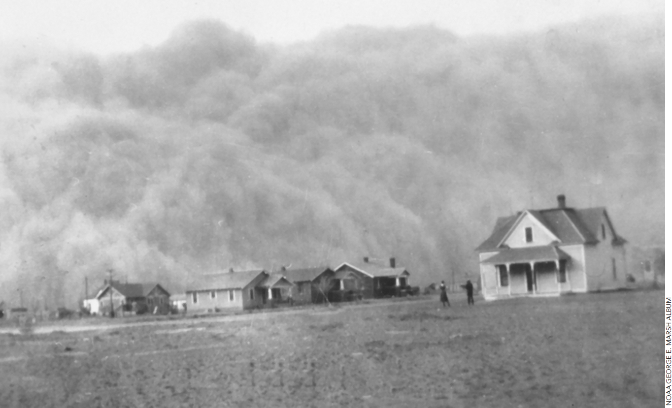
As if these shocks were not enough, the United States was beset during the early years of the Great Depression by a natural shock, namely the onset of the so-called Dust Bowl. A severe drought and decades of ecologically unsustainable farming practices turned millions of acres of farmland in Texas, Oklahoma, New Mexico, Colorado, and Kansas to dust. Dust storms blackened the sky, reducing visibility to a matter of feet. Hundreds of thousands of people were forced to leave their homes and millions of acres of farmland became useless.

In a good year, the real shocks of the Great Depression could have been absorbed without major difficulty, but in a bad year, the shocks compounded one another and made a desperate situation even worse.