CHAPTER 33 APPENDIX Business Fluctuations and the Solow Model
A way of summarizing some of the lessons of this chapter is that at least some business fluctuations are just economic growth in the short run. Economic growth happens in fits and starts rather than smoothly. The economists Finn Kydland and Edward Prescott developed key aspects of the real business cycle (RBC) model in the 1980s and were awarded the Nobel Prize for their work in 2004. One advantage of thinking about business fluctuations in this way is that they can then be analyzed using a version of the Solow growth model, which is called the real business cycle model. A complete understanding of the real business cycle model requires quite a bit of advanced mathematics, but we can briefly describe the main ideas. Consider the following production function, which is just like that used in Chapter 28 but with the addition of labor as well as capital:
Y = At × F(K, L)
To recap, output Y is a function of the inputs of capital K and labor L. In Chapter 28, we talked about the A factor as an index of ideas. Better ideas mean a larger A, which means that more output can be produced from the same inputs of capital and labor. That is a good interpretation of A in the long run, but we can also think about A as representing any factor that influences the productivity of K and L. Thus, if Y is the output of corn, then A could be deviations of rainfall from the average. Above-average rainfall, say, A = 2, means that the inputs of K and L produce a lot of corn. Below-average rainfall, say,  , means that the same inputs of K and L produce less corn.
When we are thinking about long-run economic growth, it doesn’t hurt to simplify and think about A as increasing smoothly through time. To analyze business fluctuations, however, we need to recognize that A jumps around. Thus, in the business fluctuation model, A is a productivity shock variable.
The second complication we need to add to the Solow growth model to analyze business fluctuations is to give a more sophisticated account of investment and labor supply. In the Solow growth model, investment is a simple function of output, Investment = γY, where the investment rate γ is a constant proportion like 0.3. That’s not a very realistic assumption. Will savers and investors want to invest the same proportion of output during a recession as during a boom? Probably not, for the reasons we discussed in the chapter (uncertainty, e.g.). How do savers and investors decide how much and when to invest? This is a complicated decision, requiring savers and investors to forecast future events. Solving this problem is difficult, which is where the complicated mathematics come in, but we know that γ will vary over time.
Similarly, in the growth version of the Solow model, we assumed that L was population and that L was fixed. (It’s also easy to think about L as increasing slowly and steadily.) But in the short run, we need to recognize that workers may choose to enter or exit the workforce and choose to take jobs or search for work—intertemporal substitution. As a result, L becomes the labor force and L can change due to changes in the participation rate and the unemployment rate. How do workers decide how much and when to work? Again, this is a complicated decision problem that requires workers to forecast the future and carefully optimize.
314
Adding shocks to the Solow model and giving a more sophisticated account of how savers, investors, and workers make decisions create what is known as the real business cycle model or the standard “neoclassical” model of business cycles. The intuitive account of business fluctuations that we have given in this chapter is based on this model.*
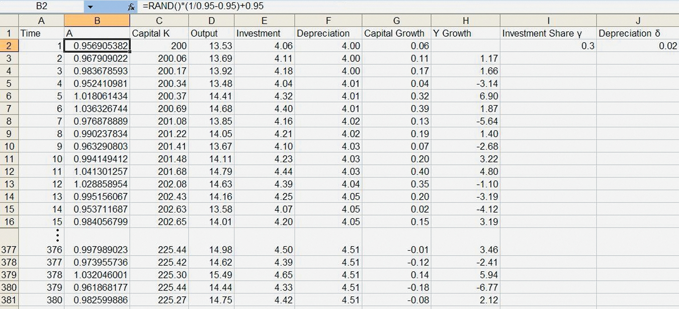
Explaining a full RBC model is too advanced for this appendix, but we recall that we showed how to simulate the Solow model using Excel in the appendix to Chapter 28. We can easily modify that model to include productivity shocks. Figure A33.1 shows our Excel model with a new column (column B) labeled A. Excel’s RAND( ) formula creates a random number between 0 and 1. If we want a number between X and Y, we can write = RAND( ) (Y – X) + X. We will use our random number as a productivity shock At , so we want a number that can be a little bigger than 1 or a little smaller than 1. Thus, when we get a random number that is greater than 1, that is a positive productivity shock (output increases), and when we get a random number that is less than 1, that is a negative productivity shock (output decreases). Thus, we input into cell B2 = RAND( )(1/0.95–0.95) + 0.95, which creates a random number between 1/0.95 and 0.95; over many draws this random number is designed so that it will average out to 1. We now modify our output formula in D2 so it reads = B2*C2^(1/2); in other words, we multiply the contribution of capital (C2^1/2) by the productivity shock At, which we generated in column B.

315
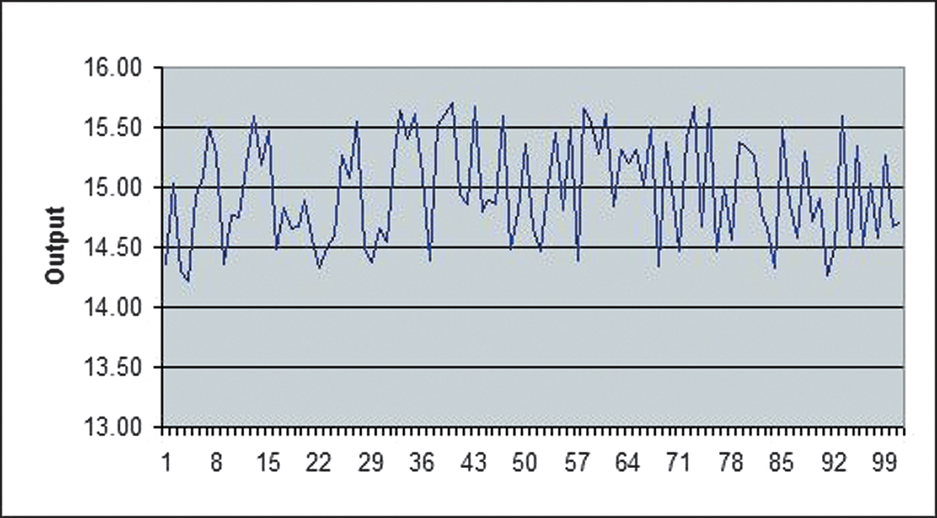
This model works very much like the Solow model in Chapter 28, but now the random shocks increase or decrease growth around the average Solow growth rate. Figure A33.2, for example, simulates 100 periods of the Solow model around the equilibrium output of 15. Notice how shocks can generate business fluctuations.

316
* For a more complete but still accessible explanation of this model, see Plosser, Charles I. Summer 1989. Understanding real business cycles. Journal of Economic Perspectives 3(3): 51–77.