CHAPTER REVIEW
FACTS AND TOOLS
Question 35.7
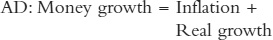
1. This chapter is concerned mostly with how monetary policy might be able to return an economy quickly to the potential growth rate after a shock. But as we saw in Chapter 31’s discussion of the quantity theory of money, a market economy has a correction mechanism to return itself slowly to the potential growth rate after a shock: flexible prices. Let’s review the quantity theory, and remember that in the quantity theory, inflation does all of the adjusting.
Recall that:  = Inflation + Real growth
Consider the nation of Kydland. Before the shock to Kydland’s economy,
 ,
,  , real growth = 4%. What is inflation?
In Kydland,
 falls to 0%, but
  stays the same. In the long run, what will inflation equal? What will real growth equal?
Consider the nation of Prescottia. Before the shock to Prescottia’s economy,
 ,
,  , real growth = 2%. What is inflation?
In Prescottia,
rises to 8%. In the long run, what will inflation equal? What will real growth equal?Consider the nation of Friedmania. Before the shock to Friedmania’s economy,
 ,
,  , real growth = 3%. What is inflation?
In Friedmania,
falls to 1%. In the long run, what will inflation equal? What will real growth equal?
Question 35.8
2. We’ve just reviewed the quantity theory of money, which is a theory that shows how the economy fixes itself in the long run. But as economist John Maynard Keynes famously said, “In the long run we are all dead.” Let’s bring SRAS back into the model, and play the role of a central banker reacting to a rise in velocity growth.
355
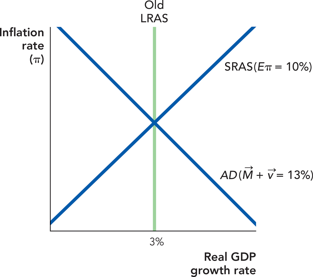
The following diagram shows the economy growing at the potential growth rate with 10% inflation. Illustrate what happens if consumers and investors become more optimistic. Clearly label the new growth rate on the x-axis with the words “High-AD real growth,” and label the new inflation rate on the y-axis with the words “High-AD inflation.”
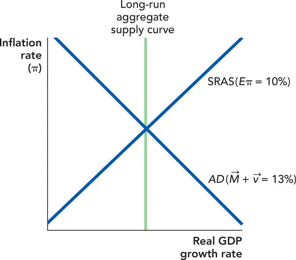
Once the central banker sees this rise in AD, she decides to fully reverse it with monetary policy. In the graph, illustrate what happens if she does her job “Just right.”
If she does her job “Just right,” what will the inflation rate be? Provide an exact number.
Question 35.9
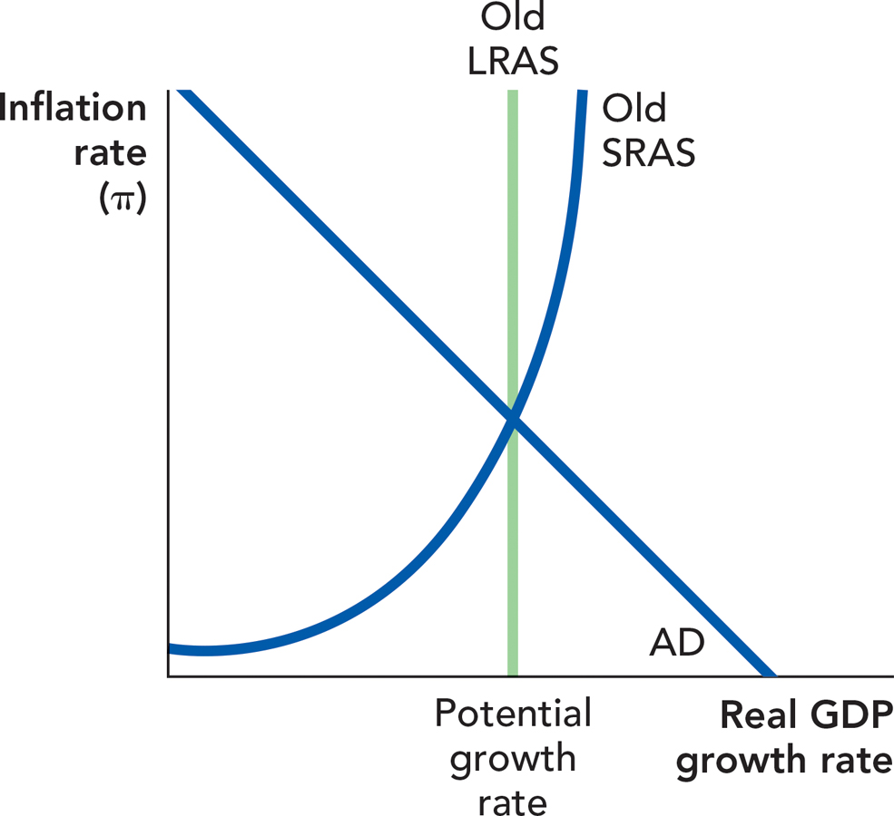
3. Let’s look at the Federal Reserve’s dilemma when there’s a positive shock to the long-run aggregate supply curve. We’ll consider the reverse of Figures 16.3 and 16.4.
In the following figure, illustrate the effect of this positive potential growth shock, ignoring the possible effect of sticky wages and prices.
If the central bank kept AD fixed, would inflation be higher or lower after this positive real shock? Would real growth be higher or lower after this positive real shock?
If the central bank wants to return inflation to its old level, should it raise money growth or lower it?
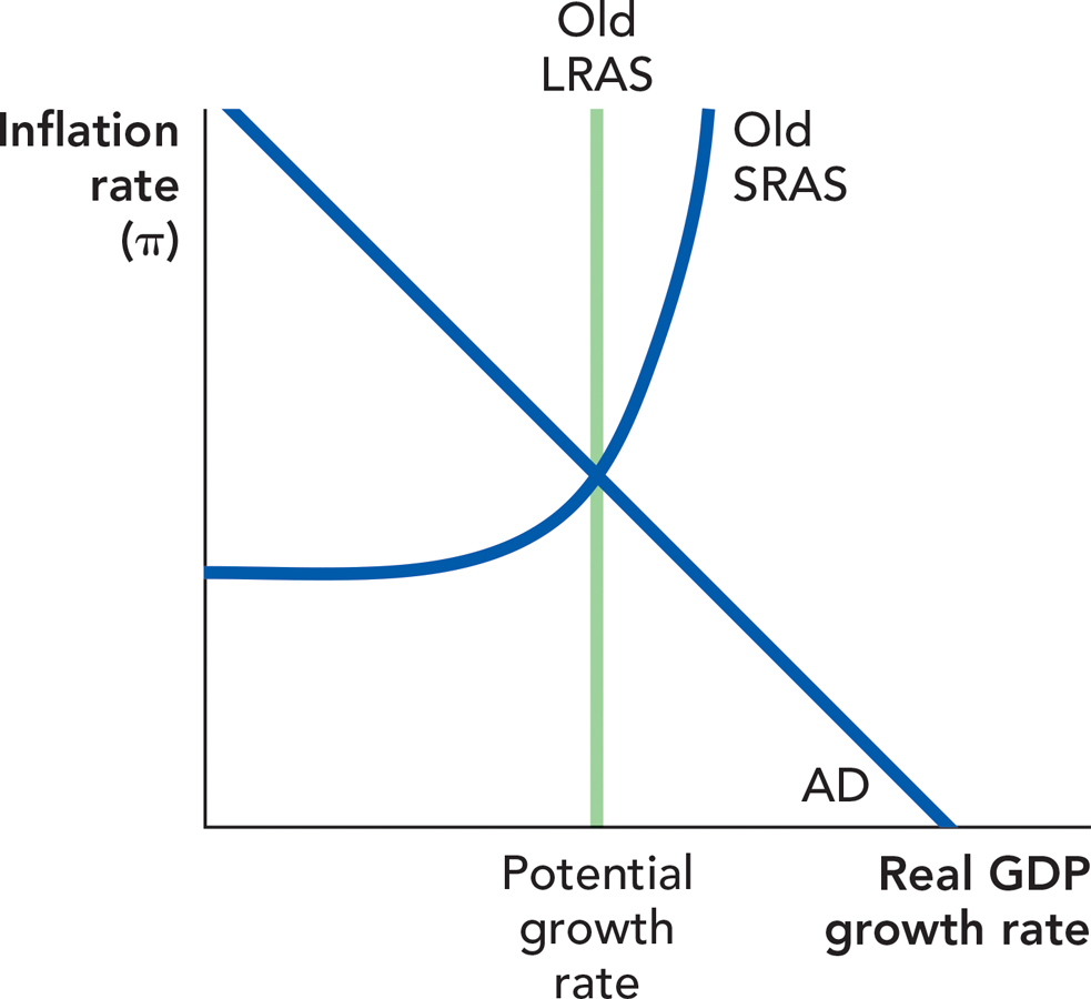
If the central bank wants to return real growth to its old level, should it raise money growth or lower it?
Economists say that central bankers face a “cruel trade-off” between inflation and real growth when a potential growth shock hits. Do your answers to parts c and d fit in with this theory?
Question 35.10
4. All of the following are called “rules.” Which of the following so-called rules are actually like “rules” and which are more like “discretion”? How can you tell the difference?
Congress passes a law providing automatic cost-of-living increases to Social Security every year. (Note: This is current U.S. law.)
Congress follows a rule to vote every few years on how much to increase Social Security payments—votes that usually occur just before an election. (This was the law before 1972.)
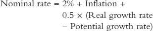
The Federal Reserve follows the famous “Taylor rule” for setting the Federal Funds rate:
The Federal Reserve follows a rule of “doing whatever seems right at the time.”
The police follow a rule of questioning anyone loitering outside of a bank who looks suspicious.
356
The police follow a rule of questioning anyone loitering outside of a bank who is dressed in bulky clothing that could conceal a weapon.
Question 35.11
5. Let’s consider a case that has some similarities to Figure 35.2. We mentioned that it’s difficult for the Fed to know what’s really happening to the economy in real time. This is similar to the well-known “fog of war,” where wartime news accounts often turn out to be exaggerations of the real story. In this question, the Federal Reserve thinks that consumer pessimism has pushed AD down by 10%, but in reality, the pessimism has pushed AD down by only 5%.
In the following figure, illustrate two AD curves: “AD with false shock” (AD-F to save room) and “AD with true shock” (AD-T).
If the central bank wants to use monetary policy to reverse a 10% shock to AD, it will have to raise money growth by 10%. Now draw two more AD curves on the figure: “Fed reacts to false shock” (FR-F to keep it short) and “Fed reacts to true shock” (FR-T).
After the central bank overreacts to the exaggerated news reports of economic calamity, what is the final result: Will real growth be higher or lower than before the shock hits? Will inflation be higher or lower than before the shock hits?
Question 35.12
6. Which of the following would be methods that the Fed could use to “maintain market confidence” when a negative AD shock hits?
Slow the growth rate of the monetary base.
Raise the interest rate on “discount window” loans.
Promise to increase the growth rate of money if the economy worsens further.
Sell Treasury bills and buy bank reserves through open market operations.
Pay a higher interest rate on reserves.
Question 35.13
7. When talking about the economy, people often make a distinction between policies that work “only in theory” compared to those that work “in practice.” In theory, a fall in money growth slows down the economy in the short run. In the six episodes since World War II when, as discussed, the Fed deliberately put the brakes on money growth, did this theory work “in practice” every single time, most of the time but not all of the time, or did this theory fail most of the time?
Question 35.14
8. A monetary policy is said to be credible if the central bank will have an incentive to do tomorrow what it says today that it will do tomorrow. Other policies may be credible or noncredible. Which of the following policies are credible?
A student promises to study for the final after going to the frat party.
A long established store offers “Guaranteed satisfaction or your money back.”
A government promises never to bail out banks that take on too much risk and go bankrupt.
Question 35.15
9.
When a financial bubble collapses, is that more like a fall in aggregate demand or a fall in the potential growth rate?
When a financial bubble collapses, what is more likely to happen as a result: a fall in inflation or a rise in inflation?
Question 35.16
10. Central banks and voters alike usually want higher real growth and lower inflation. What kind of shock makes that happen? (Note: This is similar to the type of shock that causes higher quantity and lower price in a simple supply and demand model.)
THINKING AND PROBLEM SOLVING
Question 35.17
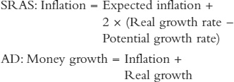
1. Let’s reenact a simplified version of the 1981— 1982 Volcker disinflation. Expected inflation and actual inflation are both 10%, real growth is 3%, and to keep it simple, velocity growth is zero. (Historical note: In fact, velocity growth shifted quite a lot during this period, which made Volcker’s job harder than in this problem. Otherwise, the numbers are close to the historical facts.) Thus, we have
357
Let’s define a simple SRAS curve:
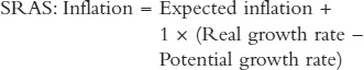
Notice that this equation gives a positive relationship between inflation and real growth for a fixed potential growth rate and expected inflation rate.
First, let’s calculate how fast the money supply grew back when inflation was 10% in 1980 and real growth was at the rate of 3%. How fast did the money supply grow at this point, before Volcker started fighting inflation? (Hint: Use the AD equation.)
Now, let’s calculate how fast Volcker will let the money supply grow in the long run, after he pulls inflation down to 4% per year. Remember, he’ll assume that in the long run, the economy will just grow at the potential growth rate. (Hint: Use AD again.)
In the short run, when Volcker cuts money growth to the rate you calculated in part b, the economy won’t grow at the potential growth rate. Instead, real output will grow at whatever rate the SRAS dictates. In terms of algebra, this means you have to combine SRAS and AD; it’s a system of two equations and two unknowns: inflation and real growth. You know the values of money growth, expected inflation, and the potential growth rate already. In the short run, what will real growth and inflation be?
Question 35.18
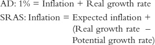
2. Now, let’s reenact the Volcker disinflation in an alternate universe where wages are more flexible and workers are much more willing to accept slower growing wages when the inflation rate falls. This will make the SRAS steeper, as we saw in our original discussion of short-run aggregate supply.
Our model economy is thus as follows:
Answer part c of the previous question again, now in this world with a steeper SRAS.
Let’s see how far this can go: What if workers pay constant attention to the Fed’s every move and will slow their wage demands the moment they see Volcker tightening the money supply? Answer the previous question with “100” in the place of “2” in the SRAS equation. Feel free to round your answers to the nearest percent.
If you were a central banker trying to cut inflation, and you want to keep real growth as close as possible to the potential growth rate, what would you prefer: a steep SRAS (i.e., workers with flexible wages), or a flatter SRAS (i.e., workers with sticky wages)?
Question 35.19
3. The Fed plays an important role in maintaining market confidence. As former Chairman Alan Greenspan put it in a 1997 address: “In [financial crises] the Federal Reserve stands ready to provide liquidity, if necessary…. The objectives of the central bank in crisis management are to … prevent a contagious loss of confidence.” [emphasis added]
Just by standing ready to provide loans to banks in an emergency, the Fed can often prevent emergencies from happening in the first place. In each of the following examples, how does the fact that someone or something stands ready to cure the bad outcome help prevent the bad outcome from ever happening in the first place?
A security guard stands inside a bank.
Federal agents guard Fort Knox, where about one-half of the U.S. government’s gold is stored.
The Federal Reserve promises to insure almost 100% of bank deposits.
Police, worried about possible riots during spring break in Palm Springs, California, bring in police from other cities.
358
Question 35.20
4. We discussed how hard it is to keep AD stable or put it back “where it belongs” after a shock. Alan Blinder, a former vice chairman of the Federal Reserve, noticed that this was a major problem. In his book Central Banking in Theory and Practice, he argued that this was a good reason for the Fed to take baby steps whenever it needed to make big shifts in AD. Sometimes you’re better off taking two years to slowly and carefully undo an AD shock rather than shift it back quickly and inaccurately in one year.
To illustrate, let’s see how things turn out if you, the central banker, take two years rather than one year to react to a negative velocity shock. You have better control over AD if you make small moves than if you make big moves, but big moves can get you back to the potential growth rate more quickly: As so often in economics, you face a trade-off.
In this question, your ultimate goal is to get AD back to 5% per year, the potential growth rate is 3%, and expected inflation is always 2% per year.
Starting point (substitute what you know into these equations and solve):
Slow approach: Add 2% per year to AD for two years (through some mix of money growth and higher confidence). What will real growth equal each year?
Start
End of Year 1
End of Year 2
Real Growth
Fast approach: Assume that you tried to add 4% to AD in Year 1, but you mistakenly add 7% instead (through some mix of excess bank lending and irrational exuberance). In the second year, you tried to correct by cutting back by 3%, but you mistakenly cut back by 4% (through some mix of slower bank lending and investors’ loss of confidence). What will real growth equal each year?
Start
End of Year 1
End of Year 2
Real Growth
You can see how the “best approach” is a matter of taste, but which method would you expect a central banker to prefer if Congress has to decide whether to reappoint the central banker to a new four-year term in a few months?
Question 35.21
5. Milton Friedman and Anna Schwartz argued in the last chapter of their Monetary History of the United States that a shift in money growth will usually cause velocity to shift in the same direction: So higher money growth causes optimism, and slower growth causes pessimism. They believed that velocity had its own shocks, as well.
Let’s run through some examples of how this might work, in a setting where the Fed wants to keep AD growth stable at 10%. To keep things simple, we’ll just assume that the Fed can control money growth perfectly, and we’ll assume that a 1% change in money growth causes a 0.5% shock to velocity growth in the same direction. Fill in the table.
In each case, AD = Initial velocity shock + Money growth + Velocity shock caused by money growth.
Year
Initial Velocity Shock
Money Growth
Velocity Shock Caused by Money Growth
1
4%
4%
4% 0.5 = 2%
2
3%
3
16%
4
8%
5
4%
6
0%
If velocity does tend to move in the direction of money growth, how does this change the Fed’s response to economic shocks: Should it take bigger moves or smaller moves in money growth when a shock comes along?
Question 35.22
6. We saw that real shocks and AD shocks often occur simultaneously. When this happens, unless we know the exact size of each shock, we can’t be sure of the effect on both inflation and real growth: We’ll know only one or the other for sure.
359
In each of the following cases, we can be sure that one of the four events will happen:
A fall in inflation
A rise in inflation
A fall in real growth
A rise in real growth
In the following cases, which changes can we confidently predict? (Hint: Draw an AD/Potential curve graph. Try several different combinations of the indicated shifts and see which outcomes are possible on the graph.)
The banking system becomes less efficient at building bridges between savers and borrowers, and investor confidence declines: A negative real shock and a negative velocity shock occur simultaneously.
The banking system becomes less efficient at building bridges between savers and borrowers, and the Federal Reserve increases money growth: A negative real shock and a positive money shock occur simultaneously.
Biologists learn how to use computer simulations to rapidly search for molecules that would make promising medicines, and investors become optimistic about future profit opportunities: A positive real shock and a positive velocity shock occur simultaneously.
Question 35.23
7. One argument for giving discretion to central bankers is that sometimes emergencies come along that a simple rule can’t solve. Suppose there’s a massive, permanent negative shock to velocity. Naturally, if the central bank has discretion, it will immediately respond by boosting money growth. But let’s look at the alternative:
Suppose that the central bank follows a fixed 3% annual monetary growth rule, as Milton Friedman sometimes recommended. In the short run, what will the velocity shock do to real growth and to inflation?
In the long run, what will this velocity shock do to real growth and to inflation?
If voters are concerned only about real growth in the long run, will they favor rules, will they favor discretion, or will they be indifferent between the two?
If voters are impatient, and concerned only about real growth in the short run, will they favor rules, will they favor discretion, or will they be indifferent between the two?
Which kind of voters favor discretion: those with a long-run horizon or those with a short-run horizon?
CHALLENGES
This chapter has more Challenge questions than usual. Take this as a sign of how difficult monetary policy really is!
Question 35.24
1. Practice with the best case: You are the central banker, and you have to decide how fast the money supply should grow. Your economy gets hit by the following AD shocks and your job is simply to neutralize them: Just push money growth in the opposite direction of the shock.
In all of the following cases, assume that there’s no change whatsoever to the potential growth rate, and assume that before the shock, you’re at your optimal inflation rate and optimal real growth rate. (Yes, this really is the best case!) These are all shocks, so think of each case study as preceded by the word, “Suddenly ….” Given the shocks to , velocity, should the central bank react by raising money growth or by cutting money growth?
Investors become pessimistic about future profit opportunities.
State governments increase spending on schools, prisons, and health care.
The federal government passes a national sales tax.
The federal government increases military spending.
Foreigners buy fewer American-made airplanes and movies.
American consumers start buying fewer domestically made Hondas and more imported Hondas.
Domestically made computers, cars, and furniture all become much more durable and longer-lasting.
Question 35.25
2. Milton Friedman famously said that changes in money growth affect the economy with “long and variable lags.” That means that if the government increases growth in the monetary base this month, the money multiplier takes a few months to turn this into growth in checking and savings deposits, and it takes a few months more before businesses and consumers actually spend this money to purchase goods and services. Let’s see how this changes our views of the previous question.
360
In each case from the previous question, the Fed predicts how long the velocity shock itself will last: We call this “shock duration” in the next table. After that time, velocity growth will go back to its old level. Additionally, in each case, the Fed’s staff of PhD economists estimates how many months it will take for a change in money supply to actually push AD in the desired direction: This is the “monetary lag.”
The question is quite simple: If monetary lags are shorter than the shock duration—if the Fed has “fair warning”—then a shift in AD will be stabilizing. If not, then a shift in AD will be like mailing a birthday card to your mother the day before her birthday: possibly destabilizing. So, in which of these cases should the Federal Reserve change money growth?
|
Case |
Monetary Lag (months) |
Shock Duration (months) |
Shift in Money Growth: Stabilizing or Destabilizing? |
|---|---|---|---|
|
a. |
14 |
8 |
|
|
b. |
18 |
12 |
|
|
c. |
20 |
Permanent |
|
|
d. |
12 |
24 |
|
|
e. |
16 |
9 |
|
|
f. |
10 |
Permanent |
|
|
g. |
18 |
Permanent |
|
Question 35.26
3. One of the reasons it’s difficult to be a monetary policymaker is because it’s so hard to tell what’s actually going on in the economy. It’s a lot like being a doctor in a world before X-rays, MRIs, and inexpensive blood tests: When the patient complains about a stomachache, you don’t know if it’s caused by food poisoning or by a tumor the size of a grapefruit.
In each of the cases from the first question, consider the fact that your data are often quite unreliable. (Fed Chair Alan Greenspan was famous for holding meetings with 100 staff economists, peppering them with questions about the quality of their data on the economy, and often knowing more than his own staff economists about the strengths and weaknesses of various surveys of the U.S. economy.) To make matters more difficult, the Federal Reserve has to forecast the behavior of Congress, which is at least as difficult as predicting the behavior of businesses: Politicians often claim they are going to raise or cut spending or taxes, but then fail to do so.
If in cases a, b, and d, the Fed chairman decides that the forecasted shocks really aren’t very likely to happen, then taking into account your answers to questions 1 and 2, in which cases should the Fed actually do nothing whatsoever in response to news about the economy?
Question 35.27
4. We explained how a central bank has an important role in maintaining confidence: “High confidence” keeps velocity growth and the money multiplier from falling. But as we’ve seen, sometimes one has to be cruel to be kind.
President Franklin Roosevelt followed this “tough love” approach during the Great Depression. Soon after taking office, he closed all banks for a four-day “bank holiday.” During this holiday, he gave his first Fireside Chat, a radio address where he explained his policies to the American people in plain language. After the four-day holiday, he still kept one-third of all U.S. banks closed (mostly small farmer banks with one or two branches). Over the next few years, only half of this one-third eventually reopened.
Thus, FDR’s bank holiday pushed the broad U.S. money supply (Ml or M2) down. Nevertheless, the economy grew quickly during FDR’s first year, 1933. Why? Because FDR promised that the banks that reopened were the safest banks, and he promised that the federal government would keep these safer banks open through generous discount window lending. This boosted confidence and encouraged people to borrow from and lend to the remaining banks.
As Milton Friedman and Anna Schwartz put it in their classic book A Monetary History of the United States; “The emergency revival of the banking system contributed to recovery by restoring confidence in the monetary and economic system and thereby inducing the public … to raise velocity … rather than by producing a growth in the stock of money” (p. 433).
361
Let’s see how an emotional concept like “confidence” shows up mathematically. To keep things simple, we’ll look at AD in terms of growth in nominal GDP (growth in dollar sales) rather than growth in real GDP (growth in actual output). We’ll compare the “before” and “after,” so we’ll skip over 1933, the year of the biggest banking crisis and of FDR’s solution to the crisis:
|
Year |
M2 |
v |
|---|---|---|
|
1932 |
$35.3 billion |
2.16 |
|
1934 |
$33.1 billion |
2.36 |
What was the level of nominal GDP in 1932 and 1934?
What was the growth of M2 between these two years?
What was the growth of velocity between these two years?
What was the growth of nominal GDP between these two years?
If velocity growth had been zero during this period (perhaps due to low confidence), but money growth stayed the same, what would have happened to nominal GDP growth?
Question 35.28
5. Central bankers often believe that their hands are tied by the public. Arthur Burns, the Fed chairman under President Nixon, reportedly said in the November 1970 Federal Reserve board meeting that “he did not believe the country was willing to accept for any long period an unemployment rate in the area of 6 percent.” In other words, if AD shocks or potential growth shocks came along that pushed the unemployment rate up, Burns believed he had to boost AD to help the economy: The voters wouldn’t tolerate anything else.
In the early 1970s, the economy was hit with some negative potential growth shocks, the most famous of which were the massive oil price increases caused by the OPEC oil embargo. Inflation started off at 4%, and Burns actually behaved according to his stated philosophy. What did Burns do to AD in the 1970s: Did he raise it or lower it?
If Burns had kept AD fixed instead of shifting it as he did, would inflation have been lower or higher than it actually turned out to be?
According to our model, did Burns’ actions raise, lower, or have no impact on the long-run aggregate supply curve?
If in the 1970s the United States had been hit by negative AD shocks instead of negative potential growth shocks, and Burns had followed his same philosophy, would inflation have been higher or lower than it actually turned out to be?
Question 35.29
6. Central bankers are reluctant to try to pop alleged bubbles. Which topics covered in this chapter might explain why they are reluctant to do so?
Question 35.30
7. We mentioned Milton Friedman’s advice that central bankers should follow a “fixed money growth rule,” where the broad money supply (M1 or M2) grows at the same rate every year. Other economists have instead recommended that central bankers follow “nominal GDP targeting,” which is similar to a fixed AD curve. Assume that the central bank really can control money growth and velocity growth within a reasonable period of time if it tries to do so.
What is the difference between a fixed money growth rule and nominal GDP targeting from the point of view of the AD equation?
If velocity shocks never occur, what’s the best policy for keeping AD as stable as possible: fixed money growth, nominal GDP targeting? Or are both equivalent?
If velocity shocks are common, what’s the best policy for keeping AD as stable as possible: fixed money growth, nominal GDP targeting? Or are both equivalent?
Question 35.31
8. The previous question assumed that the central bank can really control money growth and velocity growth within a reasonable period of time. Instead, let’s work with the more realistic assumption that it takes about a year for a change in monetary policy to actually influence money growth: Even though the central bank can increase bank reserves literally within minutes through open market operations or the term auction facility, it takes months for banks to determine whom they should lend to. And as you know, most money is created through bank loans.
362
In this question, the central bank tries to follow nominal GDP targeting so that AD grows at 7% per year. In other words, the central banks tries to set the money growth rate so that velocity growth plus money growth equals 7%. Each year, it responds to that year’s velocity growth, but the response won’t actually kick in until next year. (Think of this as driving a car with loose steering: You steer to the right, but the car only starts moving to the right about 2 seconds later.)
Fill in the following table. Notice that in each year, Actual AD = Velocity growth + Money growth. In the first year, the central bank observes velocity growth of 3% and thus targets money growth of 4%. The next year money grows at 4% as targeted, but velocity growth in that year is 1% so actual AD grows at 5%. In Year 2, the central bank observes velocity growth of 1% and thus targets money growth of 6%. Keep going.
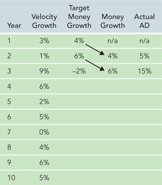
Every year, the central bank tries to keep AD = 7%, yet it never accomplishes its goal. How do “long lags” explain this failure?
How would this table look if you had followed Friedman’s 3% money growth rule instead? Don’t calculate any numbers, just answer verbally: Would the swings tend to be bigger than in the table or smaller?
Question 35.32
9.
Central bankers must manage expectations. Suppose that inflation is running at 10% and the central banker would like to lower inflation to 2% without reducing real growth. What should the central banker tell the public? And at what level should the central banker set money growth? Assume that velocity shocks are zero and that the potential growth rate is 3%.
Draw the new SRAS and AD curves.
Suppose that the public does believe the central banker. What temptation might the central banker face? (Hint: Imagine that it is an election year and the central banker would like to see the current administration reelected.)
If the central banker is not believed, what will happen? Use your answers to parts a and b to discuss the importance of independent central banks.
Question 35.33
10. In response to the housing bust and its fallout discussed at the end of this chapter, the U.S. economy entered into recession in December of 2007. That recession officially ended in June of 2009, but more than two years later at the end of 2011, many people still felt that the “recession” was not really over. As evidence, they cited high unemployment rates and the failure of some areas of the economy such as the housing market and lending to fully recover. Observers cited lack of confidence and elevated levels of uncertainty for reasons both economic and political. The Federal Reserve implemented several policies to lower both short- and long-term interest rates and increase confidence, but the private sector of the economy did not respond as it had following earlier recessions.
363
Use the AD/AS model to describe how the bursting of the housing bubble affected the economy, how the Fed responded, and the impact it had. In your discussion, be sure to point out which parts of this chapter apply to which behaviors in the economy and which parts apply to the role of the Fed in these events.
Critics of the Fed’s response in lowering and keeping interest rates so low for so long argued that the Fed was risking increased inflation. Use the AD/AS model again to explore the validity of these claims.
!launch! WORK IT OUT
In the United States, the government’s data on real growth improve over time. For instance, we now know that in the early 1970s, the economy was actually growing 4% faster than people believed. At the time, the Fed thought the economy was in a deep recession, so it mistakenly boosted money growth. The Fed’s overreaction caused inflation. Real-time surveys in the early 1970s depicted an awful economy, but as economic historians have gone back to the data, they have discovered that the economy wasn’t as awful as they thought: Someone just put the thermometer in the fridge.
Economists at the Philadelphia Federal Reserve have collected data on how our view of the economy has changed over time. These “real-time data” are summarized by Croushore and Stark in a review article entitled “A Funny Thing Happened on the Way to the Data Bank: A Real-Time Data Set for Macroeconomists” (Federal Reserve Bank of Philadelphia, Business Review, September/October 2000, 15–27). Let’s use their summary of the data and a six-sided die to see just how inaccurate our real-time views of the economy actually are.
We’re going to reenact the 1970s, and we’ll start figuring out how error-filled the government’s growth estimates will be. Croushore and Stark report that, on average:
One-sixth of the time, measured growth is 2% better than actual growth.
One-third of the time, measured growth is 1% better than actual growth.
One-third of the time, measured growth is 1.5% worse than actual growth.
One-sixth of the time, measured growth is 3% worse than actual growth.
Find a six-sided die (or use Excel to simulate rolling the die) and record your rolls in the following table. If you’ve rolled a 1, count that in category i; if you roll a 2 or 3, place that in category ii; a 4 or 5 goes in category iii; and if you roll a 6, place that in category iv. Then write down how much measurement error you’ll have for that year.
Example: If your first roll was a 4, that places you in category iii, so write down “−1.5%” as the amount of measurement error for 1971.
(Note: Psychologists and behavioral economists have found that people are fairly bad at generating truly random numbers on their own, so it’s best just to roll the die.)
Year
Roll (value)
Category
Measurement Error (%)
1971
1972
1973
1974
1975
1976
1977
1978
1979
1980
364
Let’s see what values we get when we add together the true real growth rate (which economists will only know years later) with the measurement error in the previous table. For “true real growth,” we use the most recent data in the following table—but of course even these estimates could change in the future. The sum is the actual government data that will wind up in the Federal Reserve chair’s hands.
Example: If your first roll was a 4, that placed you in category iii, so subtract 1.5% from the true 1971 growth rate to yield a real-time government report of 1.9% annual growth.
Year
True Real Growth
Government Data (%)
1971
3.4%
1972
5.3%
1973
5.8%
1974
−0.5%
1975
−0.2%
1976
5.3%
1977
4.6%
1978
5.6%
1979
3.2%
1980
−0.2%
In your simulation, how many times was the government data off by 2% or more?
If the potential growth rate in the 1970s was actually 3.6% (the average growth rate in the 1970s), then in how many years did your government data give values below 3.6% when true real growth was above 3.6%? How often did the reverse occur, with your government data above the potential rate while true real growth was below?
Add together your two values from part d. This is the number of times that even a very good central banker would have wanted to push AD in the wrong direction: it’s the number of times this weather vane was pointing in entirely the wrong direction.
(Note: You might be wondering whether the U.S. government tends to exaggerate extra good economic news just before an election. As far as economists can tell, the answer is no, at least when it comes to the official GDP number. U.S. GDP estimates contain mistakes before an election just as often as usual, but those mistakes don’t tend to favor the political party in power. In Japan, though, GDP reports do tend to be extra optimistic just before an election. For more, see Faust, Rogers, and Wright, “News and Noise in G-7 GDP Announcements,” online at the Federal Reserve Board’s Web site.)
* Recall from Chapter 26 that the exact dates of a recession are a judgment call made by the National Bureau of Economic Research. The unemployment rate is one piece of information that goes into defining when a recession begins and ends but it is quite possible for economic activity as measured by other factors such as GDP, sales, and income to be increasing even when the unemployment rate is not declining.