Fiscal Policy: The Best Case
An economic recession is under way and fear is in the air. Worried about their future, consumers cut back on consumption growth; that is,  falls. Consumers are spending less in order to build up their cash reserves so we can also say equivalently that
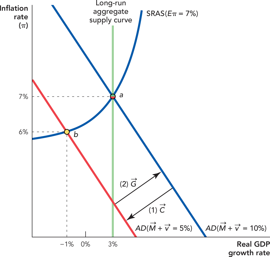
  falls. Figure 37.1 shows the result: The fall in
  shifts the AD curve to the left and down, moving the economy from a long-run equilibrium at point a to a short-run equilibrium at point b. At point b, the growth rate is negative and the economy is in a recession.
The problem at point b is that consumers want to hold more money and this means that the rate of inflation must decrease. Wages and prices, however, are sticky (see Chapter 32) so when spending growth declines, instead of just a decrease in inflation, we get a decrease in real growth as well. In terms of our AD curve, we have  = Inflation + Real growth.
  , by assumption, isn’t changing and in the short run the decrease in
  is split between a decrease in inflation and a decrease in real growth.
In the long run, prices and wages will become “unstuck,” fear will pass, and  will return to its normal growth rate so the economy will transition until it returns to point a. But recall John Maynard Keynes’s famous statement: “In the long run, we are all dead.” Can government do anything to make recovery a reality now? Quite possibly so.
Remember that the components of aggregate demand are  ,
,  ,
,  , and
, and  . The government has (some) control over
  so if
so if  falls, why not increase
  to compensate? In Figure 37.1, we show how an increase in
  can shift the AD curve to the right and up, thereby putting the economy on a transition path back to point a, reversing the decline in
  and ending the recession.
An increase in  means the government is spending more money—and thus commanding more real resources—so where does the money come from? That’s a very good question. The money must come from taxes or increased borrowing and, as we will see shortly, that will mean reduced aggregate demand from some quarters, thereby making the increase in
  less effective. But, in the best-case scenario, the increase in
  is still effective because more spending creates more growth, which supports the increased spending.

 Can Boost the Economy after
  Falls
Falls391
Can an economy really pull itself up by its bootstraps? Yes. Since John Maynard Keynes’s The General Theory of Employment, Interest and Money (1936), economists have understood that in some situations spending can increase growth, or as economists like to say, demand can create its own supply. More generally, the reason this is possible is that at point b the economy is operating inefficiently. Remember that the economy has the capital, the labor, and the technology to grow at the rate given by the long-run aggregate supply curve, so when the economy is operating at point b, it is growing at less than potential; it is growing more slowly than is possible given the fundamental factors of production. The increase in  puts the economy back on track and, if everything goes well, the increase more than pays for itself.
The Multiplier
To understand how an increase in government spending can generate growth, let’s look a little more closely at what economists call the “multiplier.” In the best-case scenario, the increase in  doesn’t even have to be as large as the fall in
  in order to restore the economy because as
  increases, so does
  . Let’s explain how this can happen.
Imagine that Joe becomes worried about unemployment so he cuts back on his daily consumption of mocha frappuccinos in an effort to hold more cash in reserve. But remember that Joe’s spending is the coffee shop owner’s income (as discussed in Chapter 26). Thus, when Joe cuts back on his spending, the coffee shop owner may cut back on her spending by, for example, hiring fewer employees or not investing in that fancy new Clover coffee machine. Thus, the decrease in Joe’s spending is added to the decrease in the coffee shop owner’s spending, which is added to the decrease in the spending of her employees and so forth. Now on an ordinary day, Joe is worried about unemployment, but Jennifer gets a new job so Joe’s reduction in consumption is matched by Jennifer’s increase and the net effect, even taking into account all the multiplier effects, is zero.
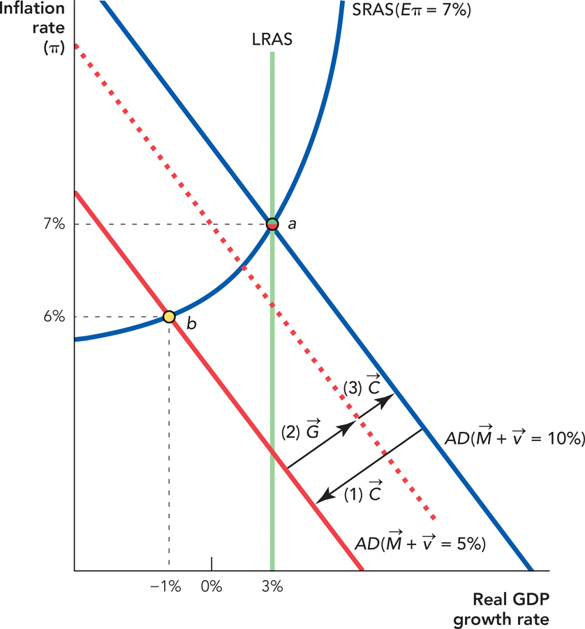
Trouble starts when a lot of people fear unemployment and reduce their spending at the same time. When many people reduce their spending, this reduces other people’s income and these people then reduce their spending and so forth in a multiplier process. But now who will act as Jennifer to restore the economy to growth? In this situation, the government may take the place of Jennifer. By spending more to build a dam, for example, the government not only increases aggregate demand directly, it also increases the income of dam workers who spend more on haircuts, which increases the income of barbers, who spend more on restaurant meals and so forth. In Figure 37.2, we show that the increase in  stimulates an increase in income and thus an increase in
  (we have drawn the figure so the net increase in AD is exactly the same as in Figure 37.1). Since the increase in
  multiplies the effect of expansionary fiscal policy on AD, this effect is called the multiplier effect.

 stimulates
  so the increase in AD can be larger than the increase in
  alone.
The multiplier effect is the additional increase in AD caused when expansionary fiscal policy increases income and thus consumer spending.
392
All of this sounds great. The government can offset decreases in AD with increases in  and because of the multiplier effect, it doesn’t even have to spend that much. As you probably expected, however, the real world isn’t quite so simple.
CHECK YOURSELF
Question 37.1
 What are the two types of expansionary fiscal policy?