The Elasticity of Demand
The elasticity of demand measures how responsive the quantity demanded is to a change in price; more responsive equals more elastic.
When the price of a good increases, individuals and businesses will buy less. But how much less? A lot or a little? The elasticity of demand measures how responsive the quantity demanded is to a change in price—the more responsive quantity demanded is to a change in the price, the more elastic is the demand curve. Let’s start by comparing two different demand curves.
In Figure 5.1, when the price increases from $40 to $50, the quantity demanded decreases from 100 to 20 along demand curve E but only from 100 to 95 along demand curve I—thus, demand curve E is more elastic than demand curve I.
Elasticity is not the same thing as slope, but they are related and for our purposes you won’t make any mistakes if you follow the elasticity rule:
Elasticity rule: If two linear demand (or supply) curves run through a common point, then at any given quantity the curve that is flatter is more elastic.
Determinants of the Elasticity of Demand
Of the two curves in Figure 5.1, which do you think would best represent the demand curve for oil?

There are few substitutes for oil in its major use, transportation, so when the price increases by a lot, the quantity demanded falls by only a little. Thus, the demand curve for oil is not very elastic and would be best represented by demand curve I.
The fundamental determinant of the elasticity of demand is how easy it is to substitute one good for another. The fewer substitutes for a good, the less elastic the demand. The more substitutes for a good, the more elastic the demand.
69
When the price of oil goes up, people grumble but few stop using cars, at least not right away. But what happens to the elasticity of the demand for oil over time? The demand for oil tends to become more elastic over time because the more time people have to adjust to a price change, the better they can substitute one good for another. In other words, there are more substitutes for oil in the long run than in the short run. Since the OPEC oil price increases in the 1970s (see Figure 4.9 in Chapter 4), the U.S. economy has slowly substituted away from oil by moving toward other sources of energy such as coal, nuclear, and hydroelectric. It took many years, but today the U.S. economy uses about half the amount of oil per dollar of GDP than it did in the 1970s.1
In the long run, there are even substitutes for oil in transportation. One reason that mopeds are more popular and SUVs less popular in Europe than in the United States is that taxes make the price of gasoline much higher in Europe than in the United States. Europeans have adjusted by buying more mopeds and smaller cars and driving fewer miles—Americans would do the same if the price of gasoline were expected to increase permanently.
If the price of oil increases by a significant amount for a long period, then even the organization of cities will change as people move from suburbia toward apartments and townhouses located closer to work. It may seem odd to think of moving closer to work as a “substitute for oil,” but people adjust to price increases in many ways and economists think of all these adjustments as involving substitutes. If the price of cigarettes goes up and people decide to satisfy their oral cravings by chewing carrots, then carrots are a substitute for cigarettes.
In short, the more time people have to adjust to a change in price, the more elastic the demand curve will be.
Let’s compare the demand for Orange Crush, a particular brand of orange soda, with the demand for orange soda. There are many good substitutes for Orange Crush, including Orangina, Fanta, and Slice (Wikipedia lists 24 types of orange soda). As a result, the demand for Orange Crush is very elastic because even a small increase in the price of Orange Crush will result in a large decrease in the quantity demanded as people switch to the substitutes. The demand curve for orange soda, however, is less elastic because there are fewer substitutes for orange soda than there are for Orange Crush and the substitutes such as root beer or cola are not as good. We illustrate this in Figure 5.2. The general point is that the demand for a specific brand of a product is more elastic than the demand for a product category. We will come back to this point when we look in more depth at competition and monopoly in Chapter 12 and Chapter 13.

What counts as a good substitute depends on a buyer’s preferences, as well as on objective properties of the good. If the price of Coca-Cola increases at the supermarket, many people will buy Pepsi but others will keep on buying Coca-Cola because for them Pepsi is not a good substitute. So, some people have a more elastic demand for Coca-Cola, while other people have a less elastic demand. A closely related idea is that demand is less elastic for goods that people consider to be “necessities” and is more elastic for goods that are considered “luxuries.” Of course, for some people their morning coffee at Starbucks is a necessity and for others it’s a luxury. Let’s summarize by saying that the demand for necessities—however a person defines that term—tends to be less elastic and the demand for luxuries tends to be more elastic.
70
The higher a person’s income, the less concerned they are likely to be with the price of an item; thus, higher income makes demand less elastic. In 2008, the price of wheat tripled, and many people all around the world bought less bread. But neither of the authors of this book cut back much on his consumption of bread. The price of bread is too small a portion of our budgets to worry very much about its price, so our consumption of bread is not very elastic. On the other hand, when the price of housing increases, we buy smaller houses just like everyone else. Thus, the larger the share of a person’s budget devoted to a good, the more elastic his or her demand for that good is likely to be. We summarize the determinants of the elasticity of demand in Table 5.1.
TABLE 5.1 Some Factors Determining the Elasticity of Demand
|
Less Elastic |
More Elastic |
|---|---|
|
Fewer substitutes |
More substitutes |
|
Short run (less time) |
Long run (more time) |
|
Categories of product |
Specific brands |
|
Necessities |
Luxuries |
|
Small part of budget |
Large part of budget |
Calculating the Elasticity of Demand
The elasticity of demand has a precise definition with important properties. The elasticity of demand is the percentage change in the quantity demanded divided by the percentage change in price.
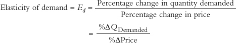
where Δ (delta) is the mathematical symbol for “change in.”
 If the price of oil increases by 10% and over a period of several years the quantity demanded falls by 5%, then the long-run elasticity of demand for oil is −5%/10% = −0.5, or 0.5 in absolute terms.
If the price of Minute Maid orange juice falls by 10% and the quantity of Minute Maid orange juice demanded increases by 17.5%, then the elasticity of demand for Minute Maid OJ is 17.5%/−10% = −1.75, or 1.75 in absolute terms.2
Elasticities of demand are always negative because when the price goes up, the quantity demanded always goes down (and vice versa), which is why economists sometimes drop the negative sign and work with the absolute value instead.
When the absolute value of the elasticity is less than 1, the demand is not very elastic or economists say the demand is inelastic; if it is greater than 1, economists say that demand is elastic; and if it is exactly equal to 1, economists say that demand is unit elastic. So in our calculations, oil has inelastic demand and Minute Maid orange juice has elastic demand.
The elasticity of demand is a measure of how responsive the quantity demanded is to a change in price. It is computed by

|Ed| > 1 = Elastic
|Ed| < 1 = Inelastic
|Ed| = 1 = Unit elastic
Using the Midpoint Method to Calculate the Elasticity of Demand To calculate an elasticity, you need to know how to calculate the percentage change in quantity and the percentage change in price. That is a bit trickier than it sounds. To see why, let’s suppose that you observe the price and quantity pairs shown in the table (careful readers will note that these points correspond to points a and b along demand curve E in Figure 5.1).
71
If you think of moving from point a to point b (let’s call this moving from “before” to “after”), then the quantity demanded falls from 100 to 20 so the change in quantity demanded is −80. What is the percentage change in quantity demanded?
|
|
Price |
Quantity Demanded |
|---|---|---|
|
Point a |
$40 |
100 |
|
Point b |
$50 |
20 |
If the beginning quantity, QBefore, is 100 and the ending quantity, QAfter, is 20, it seems natural to calculate the percentage change in quantity like this:

But now think of moving from point b to point a. In this case, quantity demanded increases from 20 to 100 and it now seems natural to calculate the percentage change in quantity like this:
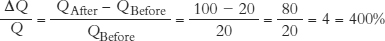
In the first case, we are thinking of a percentage decrease in quantity and in the second of a percentage increase in quantity so it’s easy to see why one number is negative and the other positive. But why are the numbers so different when we are calculating exactly the same change?
The different values occur because the base of the calculation changes. If you are driving 100 mph and decrease speed to 20 mph, it’s natural to say that your speed went down by 80% because you calculate using a base of 100. But if you are driving 20 mph and you increase speed to 100 mph, it’s natural to say that you increased your speed by 400% since you now use 20 as the base. Economists would like to calculate the same number for elasticity whether the quantity (or speed) decreases from 100 to 20 or increases from 20 to 100.
To avoid problems with the choice of base, economists calculate the percentage change in quantity by dividing the change in quantity by the average or midpoint quantity—the base is thus the same whether you think about quantity as increasing or decreasing.
Here is the formula:
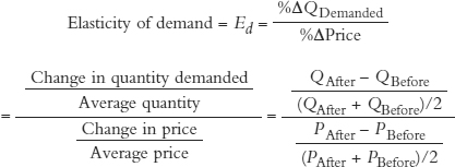
In this case, we calculate the percentage change in quantity demanded as 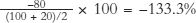 , and we also use the midpoint formula for the percentage change in price, which is
 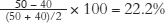 . With these two numbers, we can now calculate the elasticity of demand over this portion of the demand curve:
72
Notice that the absolute value of the elasticity, 6, is greater than 1, so the demand is elastic over this range.
It’s most important that you understand the concept of elasticity. To calculate an elasticity, don’t worry too much; just remember where the formula is located and plug in the numbers. In the second appendix to this chapter, we show how to create a simple Excel spreadsheet to calculate elasticity so you need not even worry about making calculation mistakes (at least not on your homework!).
Total Revenues and the Elasticity of Demand
A firm’s revenues are equal to price per unit times quantity sold.
Revenue = Price × Quantity, or R = P × Q
Elasticity measures how much Q goes down when P goes up, so you might suspect that there is a relationship between elasticity and revenue. Indeed, the relationship is remarkably useful: If the demand curve is inelastic, then revenues go up when the price goes up. If the demand curve is elastic, then revenues go down when the price goes up.
Let’s give some intuition for this result. Imagine that the demand curve is inelastic, thus not responsive to price. This means that when P goes up by a lot, Q goes down by a little, like this

So when the demand curve is inelastic, what will happen to revenues? If P goes up by a lot and Q goes down by a little, then revenues will go up

Thus, when the demand curve is inelastic, revenues go up when the price goes up and, of course, revenues will go down when the price goes down.
We can also show the relationship in a diagram. Figure 5.3 shows an inelastic demand curve on the left and an elastic demand curve on the right.* Revenue is P × Q, so revenue is equal to the area of a rectangle with height equal to price and width equal to the quantity; for example, when the price is $40 and the quantity is 100, revenues are $4,000, or the area of the blue rectangle (note that the blue and green rectangles overlap).

In both diagrams, the blue rectangles show revenue at a price of $40 and the green rectangles show revenues at the higher price of $50. Compare the size of the blue and green rectangles when the demand curve is inelastic (on the left) and when the demand curve is elastic (on the right). What do you see? When the demand curve is inelastic, an increase in price increases revenues (the green rectangle is bigger than the blue rectangle), but when the demand curve is elastic, an increase in price decreases revenues (the green rectangle is smaller than the blue rectangle).
73
Of course, the relationships hold in reverse as well. If the demand curve is inelastic, a price decrease causes a decrease in revenues, and if the demand curve is elastic, a price decrease causes an increase in revenues.
Can you guess what happens to revenues when price increases or decreases and the demand curve is unit elastic? Right, nothing! When the demand curve is unit elastic, a change in price is exactly matched by an equal and opposite percentage change in quantity so revenues stay the same. Unit elasticity is the dividing point between elastic and inelastic curves.
You should be able to use all of these relationships on an exam. Table 5.2 summarizes what we have covered so far.
TABLE 5.2 Elasticity and Revenue
|
Absolute Value of Elasticity |
Name |
How Revenue Changes with Price |
|---|---|---|
|
|Ed| < 1 |
Inelastic |
Price and revenue move together. |
|
|Ed| > 1 |
Elastic |
Price and revenue move in opposite directions. |
|
|Ed| = 1 |
Unit elastic |
When price changes, revenue stays the same. |
74
If you must, memorize the table. At least one of your textbook authors, however, can never remember the relationship between elasticity and total revenue. So, instead of memorizing the relationship, he always derives it by drawing little diagrams like those in Figure 5.3. If you can easily duplicate these diagrams, you too will always be able to answer questions involving elasticity and total revenue.