Price Ceilings
Nixon’s price controls didn’t have much effect immediately because prices were frozen near market levels. But the economy is in constant flux and market prices soon shifted. At the time of the freeze, prices were rising because of inflation, so the typical situation came to resemble that in Figure 8.1, with the controlled price below the uncontrolled or market equilibrium price.
FIGURE 8.1

When the maximum price that can be legally charged is below the market price, we say that there is a price ceiling. Economists call it a price ceiling because prices cannot legally go higher than the ceiling. Price ceilings create five important effects:
Shortages
Reductions in product quality
Wasteful lines and other search costs
A loss of gains from trade
A misallocation of resources
A price ceiling is a maximum price allowed by law.
Shortages

When prices are held below the market price, the quantity demanded exceeds the quantity supplied. Economists call this a shortage. Figure 8.1 shows that the shortage is measured by the difference between the quantity demanded at the controlled price and the quantity supplied at the controlled price. Notice also that the lower the controlled price is relative to the market equilibrium price, the larger the shortage.
In some sectors of the economy, shortages appeared soon after prices were controlled in 1971. Increased demand in the construction industry, for example, meant that price controls hit that sector especially hard. Ordinarily, increased demand for steel bars, for example, would increase the price of steel bars, encouraging more production. But with a price ceiling in place, demanders could not signal their need to suppliers nor could they provide suppliers with an incentive to produce more. As a result, shortages of steel bars, lumber, toilets (for new homes), and other construction inputs were common. By 1973, there were shortages of wool, copper, aluminum, vinyl, denim, paper, plastic bottles, and more.
Reductions in Quality
At the controlled price, demanders find that there is a shortage of goods—they cannot buy as much of the good as they would like. Equivalently, at the controlled price, sellers find that there is an excess of demand or, in other words, sellers have more customers than they have goods. Ordinarily, this would be an opportunity to profit by raising prices, but when prices are controlled, sellers can’t raise prices without violating the law. Is there another way that sellers can increase profits? Yes. It’s much easier to evade the law by cutting quality than by raising price, so when prices are held below market levels, quality declines.

C. Jackson Grayson, chairman of the U.S. Price Commission, was worried about the bad publicity, so on Face the Nation he triumphantly held aloft a can of Mrs. Adler’s soup claiming that his staff had opened many cans and concluded there were still four balls per can.
Whoever was right about the soup, Meany was certainly the better economist: Price ceilings reduce quality.
Thus, even when shortages were not apparent, quality was reduced. Books were printed on lower-quality paper, 2″ × 4″ lumber shrank to  , and new automobiles were painted with fewer coats of paint. To help deal with the shortage of paper, some newspapers even switched to a smaller font size.1
Another way quality can fall is with reductions in service. Ordinarily, sellers have an incentive to please their customers, but when prices are held below market levels, sellers have more customers than they need or want. Customers without potential for profit are just a pain so when prices cannot rise, we can expect service quality to fall. The full service gasoline station, for example, disappeared with price controls in 1973, and instead of staying open for 24 hours, gasoline stations would close whenever the owner wanted a lunch break.
Wasteful Lines and Other Search Costs
The most serious shortage during the 1970s was for oil. The OPEC embargo in 1973 and the reduction in supply caused by the Iranian Revolution in 1979 increased the world price of oil, as we saw in Chapter 4. In the United States, however, price controls on domestically produced oil had not been lifted and thus the United States faced intense shortages of oil and the classic sign of a shortage, lines.
Figure 8.2 focuses on the third consequence of controlling prices below market prices: wasteful lines.
FIGURE 8.2

At the controlled price of $1, sellers supply Qs units of the good. How much are demanders willing to pay (per unit) for these Qs units? Recall that the demand curve shows the willingness to pay, so follow a line from Qs up to the demand curve to find that demanders are willing to pay $3 per unit for Qs units. The price controls, however, make it illegal for demanders to offer sellers a price of $3, but there are other ways of paying for gas.
Knowing that there is a shortage, some buyers might bribe station owners (or attendants) to fill up their tanks. Suppose that the average tank holds 20 gallons. Buyers would then be willing to pay $60 for a fill-up, the legal price of $20 plus a $40 under-the-table bribe. Thus, if bribes are common, the total price of gasoline—the legal price plus the bribe price—will rise to $3 per gallon ($60/20 gallons).

Corruption and bribes can be common, especially when price controls are long-lasting, but they were not a major problem during the gasoline shortages of the 1970s. Nevertheless, the total price of gasoline did rise well above the controlled price. Instead of competing by paying bribes, buyers competed by their willingness to wait in line. Remember that at the controlled price the quantity of gasoline demanded is greater than the quantity supplied, so some buyers are going to be disappointed—they are going to get less gasoline than they want and some buyers may get no gasoline at all. Buyers will compete to avoid being left with nothing. Let’s assume that all gasoline station owners refuse bribes. Unfortunately, honesty does not eliminate the shortage. A first-come/first-served system is honest, but buyers who get to the gasoline station early will get the gas, leaving the latecomers with nothing. In this situation, how long will the lineups get?
Suppose that buyers value their time at $10 an hour and, as before, the average fuel tank holds 20 gallons. Eager to obtain gas during the shortage, a buyer arrives at the station early, perhaps even before it opens, and must wait in line for an hour before he is served. His total price of gas is $30: $1 per gallon for 20 gallons in out-of-pocket cost plus $10 in time cost. Since the total value of the gas is $60, that’s still a good deal. But if it’s a good deal for him, it’s probably a good deal for other buyers, too, so the next time he wants to fill up, he is likely to discover that others have preceded him and now he has to wait longer. How much longer? Following the logic to its conclusion, we can see that the line will lengthen until the total cost for 20 gallons of gasoline is $60: $20 in cash paid to the station owner plus $40 in time costs (4 hours worth of waiting). The price per gallon, therefore, rises to $3 ($60/20 gallons)—exactly as occurred with bribes!
Price controls do not eliminate competition. They merely change the form of competition. Is there a difference between paying in bribes and paying in time? Yes. Paying in time is much more wasteful. When a buyer bribes a gasoline station owner $40, at least the gasoline station owner gets the bribe. But when a buyer spends $40 worth of time or four hours waiting in line, the gasoline station owner doesn’t get to add four hours to his life. The bribe is transferred from the buyer to the seller, but the time spent waiting in line is simply lost. Figure 8.2 shows that when the quantity supplied is Qs, the total price of gasoline will tend to rise to $3: a $1 money price plus a time-price of $2 per gallon. The total amount of waste from waiting in line is given by the shaded area, the per gallon time price ($2) multiplied by the number of gallons bought (Qs).*
Lost Gains from Trade (Deadweight Loss)
Price controls also reduce the gains from trade. In Figure 8.3, at the quantity supplied Qs, how much would demanders pay for one additional gallon of gasoline? The willingness to pay for a gallon of gas at Qs is $3, so demanders would be willing to pay just a little bit less, say, $2.95, for an additional gallon. How much would suppliers require to sell an additional gallon? Supplier cost is read off the supply curve, so reading up from the quantity Qs to the supply curve, we find that the willingness to sell at Qs is $1; suppliers would be willing to supply an additional unit for just a little bit more, say, $1.05.
FIGURE 8.3

A deadweight loss is the total of lost consumer and producer surplus when not all mutually profitable gains from trade are exploited. Price ceilings create a deadweight loss.
Demanders are willing to pay $2.95 for an additional gallon of gas, suppliers are willing to sell an additional gallon for $1.05, and so there is $1.90 of potential gains from trade to split between them. But it’s illegal for suppliers to sell gasoline at any price higher than $1. Buyers and sellers want to trade, but they are prevented from doing so by the threat of jail. If the price ceiling were lifted and trade were allowed, the quantity traded would expand from Qs to Qm and buyers would be better off by the green triangle labeled “Lost consumer surplus,” while sellers would be better off by the blue triangle labeled “Lost producer surplus.” But with a price ceiling in place, the quantity supplied is Qs and together the lost consumer and producer surplus are lost gains from trade (economists also call this a deadweight loss).
Recall from Chapter 4 that we said that in a free market the quantity of goods sold maximizes the sum of consumer and producer surplus. We can now see that in a market with a price ceiling, the sum of consumer and producer surplus is not maximized because the price control prevents mutually profitable gains from trade from being exploited.
In addition to these losses, price controls cause a misallocation of scarce resources; let’s see how that works in more detail.
Misallocation of Resources
In Chapter 7, we explained how a price is a signal wrapped up in an incentive. Price controls distort signals and eliminate incentives. Imagine that it’s sunny on the West Coast of the United States, but on the East Coast a cold winter increases the demand for heating oil. In a market without price controls, the increase in demand in the East pushes up prices in the East. Eager for profit, entrepreneurs buy oil in the West, where the oil is not much needed and the price is low, and they move it to the East, where people are cold and the price of oil is high. In this way, the price increase in the East is moderated and supplies of oil move to where they are needed most.
Now consider what happens when it is illegal to buy or sell oil at a price above a price ceiling. No matter how cold it gets in the East, the demanders of heating oil are prevented from bidding up the price of oil, so there’s no signal and no incentive to ship oil to where it is needed most. Price controls mean that oil is misallocated. Swimming pools in California are heated, while homes in New Jersey are cold. In fact, this was exactly what happened in the United States, especially in the harsh winter of 1972–1973.
Once again recall from Chapter 4 that we said that in a free market the supply of goods is bought by the demanders who have the highest willingness to pay. We can now see that in a market with a price ceiling, demanders with the highest willingness to pay have no easy way to signal their demands nor do suppliers have an incentive to supply their demands. As a result, in a controlled market goods are misallocated.
Price controls cause resources to be misallocated not just geographically, but also across different uses of oil. Recall from Chapter 3 that the demand curve for oil shows the uses of oil from the highest-valued to the lowest-valued uses. In case you forgot, Figure 8.4 shows the key idea: High-valued uses are at the top of the curve and low-valued uses at the bottom. Without market prices, however, we have no guarantee that oil will flow to its highest-valued uses. As we have just seen, in a situation with price controls, it’s possible to have plenty of oil to heat swimming pools in California (hello, rubber ducky!) and not enough oil for heating cold homes in New Jersey. Similarly, in 1974 Business Week reported, “While drivers wait in three-hour lines in one state, consumers in other states are breezing in and out of gas stations.”2
FIGURE 8.4

Figure 8.5 illustrates the problem more generally. As we know, at the controlled price, the quantity demanded Qd exceeds the quantity supplied Qs and there is a shortage. Ideally, we would like to allocate the quantity of oil supplied Qs, to its highest-valued uses; these are illustrated at the top of the demand curve by the thick line. But the potential consumers of the oil with the highest-valued uses are legally prevented from signaling their high value by offering to pay oil suppliers more than the controlled price. Oil suppliers, therefore, have no incentive to supply oil to just the highest-valued uses. Instead, oil suppliers will give the oil to any user who is willing to pay the controlled price—but most of these users of oil have lower-valued uses. Like the lines at the gas station, it’s first-come/first-served. In fact, the only uses of oil that definitely will not be satisfied are the least-valued uses. (Why not? The users with the least-valued uses are not even willing to pay the controlled price.)
FIGURE 8.5

When a crisis in the Middle East reduces the supply of oil, the price system rationally responds by reallocating oil from lower-valued uses to the highest-value uses. In contrast, when the supply of oil is reduced and there are price ceilings, oil is allocated according to random and often trivial factors. The shortage of heating oil in 1971, for example, was exacerbated by the fact that President Nixon happened to impose price controls in August when the price of heating oil was near its seasonal low.3 Since the price of heating oil was controlled at a low price, while gasoline was controlled at a slightly higher price, it was more profitable to turn crude oil into gasoline than into heating oil. As winter approached, the price of heating oil would normally have risen and refiners would have turned away from gasoline production to the production of heating oil, but price controls removed the incentive to respond rationally.
Advanced Material: The Loss from Random Allocation If there were no misallocation, then under a price control consumer surplus would be the area between the demand curve and the price up to the quantity supplied, the green area in Figure 8.6. (Of course, some of this surplus will likely be eaten up by bribes, time spent waiting in line, and so forth as explained earlier.)
FIGURE 8.6

Under a price control, however, the good is not necessarily allocated to the highest-valued uses. As a result, consumer surplus will be less than the green area—but how much less? The worst-case scenario would occur if all the goods were allocated to the lower-valued uses, but that seems unlikely. A more realistic assumption is that under price controls, goods are allocated randomly so that a high-valued use is as likely as a low-valued use to be satisfied.
In Figure 8.7 we show two uses. The highest-valued use has a value of $30 and the lowest-valued use has a value of $6. Now imagine that one unit of the good is allocated randomly between these two uses. Thus, with a probability of 1/2, it will be allocated to the use with a value of 30, and with a probability of 1/2, it will be allocated to the use with a value of 6. On average, how much value will this unit create? The average value will be
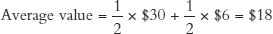
FIGURE 8.7

Extending this logic, it can be shown that if every use between the highest-valued use and the lowest-valued use is equally likely to be satisfied, then the average value is $18. Thus on average, a randomly allocated unit of the good will create a value of $18. If there are, say, 10 units allocated, then the total value of those units will be 10 × $18 = $180. Since the average value is $18 and the controlled price is $6, consumer surplus is the green area in Figure 8.7 labeled total consumer surplus under random allocation. But notice that the green area in Figure 8.7, consumer surplus under random allocation, is much less than the green area in Figure 8.6, consumer surplus under allocation to the highest value uses. The difference is the red area in Figure 8.7, the loss due to random allocation.
Misallocation and Production Chaos Shortages in one market create breakdowns and shortages in other markets, so the chaos of price controls expands even into markets without price controls. In ordinary times, we take it for granted that products will be available when we want them, but in an economy with many price controls, shortages of key inputs can appear at any time. In 1973, for example, million-dollar construction projects were delayed because a few thousand dollars worth of steel bar was unavailable.4
Perhaps the height of misallocation occurred when shortages of steel drilling equipment made it difficult to expand oil production; this mistake took place even as the United States was undergoing the worst energy crisis in its history.5
As the shortages and misallocations grew worse, schools, factories, and offices were forced to close, and the government stepped in to allocate oil by command. President Nixon ordered gasoline stations to close between 9 pm Saturday and 12:01 am Monday.6 The idea was to prevent “wasteful” Sunday driving, but the ban simply encouraged people to fill their tanks earlier. Daylight savings time and a national 55-mph speed limit were put into place (the latter not to be repealed until 1995). Some industries, such as agriculture, were given priority treatment for fuel allocation, while others were forced to endure cutbacks. Fuel for noncommercial aircraft, for example, was cut by 42.5% in November of 1973, sending the local economy of Wichita, Kansas, where aircraft producers Cessna, Beech, and Lear were located, into a tailspin.7
Some of these ideas for conserving fuel were probably sensible while others were not, but without market prices, it’s hard to tell which is which. The subtlety of the market process in allocating oil and taking advantage of links between markets is difficult, even impossible, to duplicate. C. Jackson Grayson was chairman of President Nixon’s Price Commission, but after seeing how controls worked in practice, he said:
Our economic understanding and models are simply not powerful enough to handle such a large and complex economic system better than the marketplace.8
The End of Price Ceilings
CHECK YOURSELF
Question 8.1
![]() Nixon’s price controls set price ceilings below the market price. What would have happened if the price ceilings had been set above market prices?
Nixon’s price controls set price ceilings below the market price. What would have happened if the price ceilings had been set above market prices?
Question 8.2
![]() Under price controls, why were the shortages of oil in some local markets much more severe than in others?
Under price controls, why were the shortages of oil in some local markets much more severe than in others?
Price controls for most goods were lifted by April 1974, but controls on oil remained in place. Over the next seven years, controls on oil would be eased but at the price of substantial increases in complexity and bureaucracy. In September 1973, for example, price controls were lifted on new oil. “New oil” was defined as oil produced on a particular property in excess of the amount that had been produced in 1972. Decontrol of new oil was a good idea because it increased the incentive to develop new deposits. The two-tier system, however, also created wasteful gaming as firms shut down some oil wells only to drill “new” wells right next door.9 The battle between entrepreneurs and regulators was met with increasingly complex rules. Thus, the two-tier program was extended to three tiers, then five, then eight, then eleven.
Price controls on oil ended as abruptly as they had begun when on the morning of January 20, 1981, Ronald Reagan was inaugurated as president, and before lunch with Congress, he performed his first act as president—eliminating all controls on oil and gasoline. As expected, the price of oil in the United States rose a little but the shortage ended overnight. Within a year, prices began to fall as supply increased and within a few years they were well below the levels of 1979. Fluctuations in the price of oil have continued to occur, of course, but since the ending of controls, there has been no shortage of oil in the United States.