We learned in Chapter 7 and Chapter 8 that economic growth depends on increases in the stocks of labor and capital and on increases in productivity (driven by new and better ideas and better institutions). Thus, every economy has a potential growth rate given by these fundamental, or real, factors of production. We call the rate of growth, as given by the real factors of production, the “Solow” growth rate. We call it that because Robert Solow, one of the giants of economics, created an important model of an economy’s fundamental growth rate. In Chapter 8, we described Solow’s model in more detail, but if you skipped that section don’t worry: Just think of the Solow growth rate as the rate of economic growth given flexible prices and the existing real factors of capital, labor, and ideas.

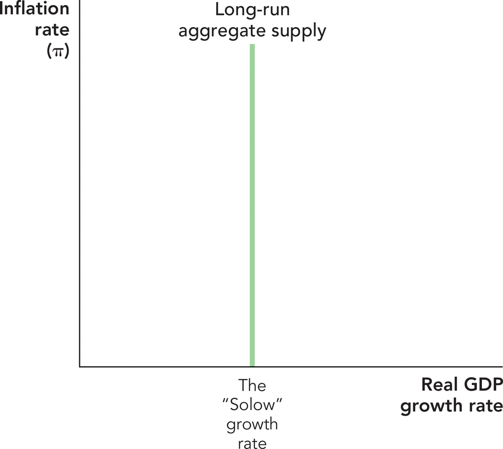
In the long run money is neutral, as we emphasized in Chapter 12. Thus, when we put the inflation rate on the vertical axis of a graph and real growth (the growth rate of real GDP) on the horizontal axis, the long-run aggregate supply curve is very simple—it’s a vertical line at the Solow growth rate. Figure 13.5 illustrates the long run aggregate supply curve.* Once again, the fundamental growth rate of the economy depends on factors such as the amount and quality of labor and capital, not on the rate of inflation.

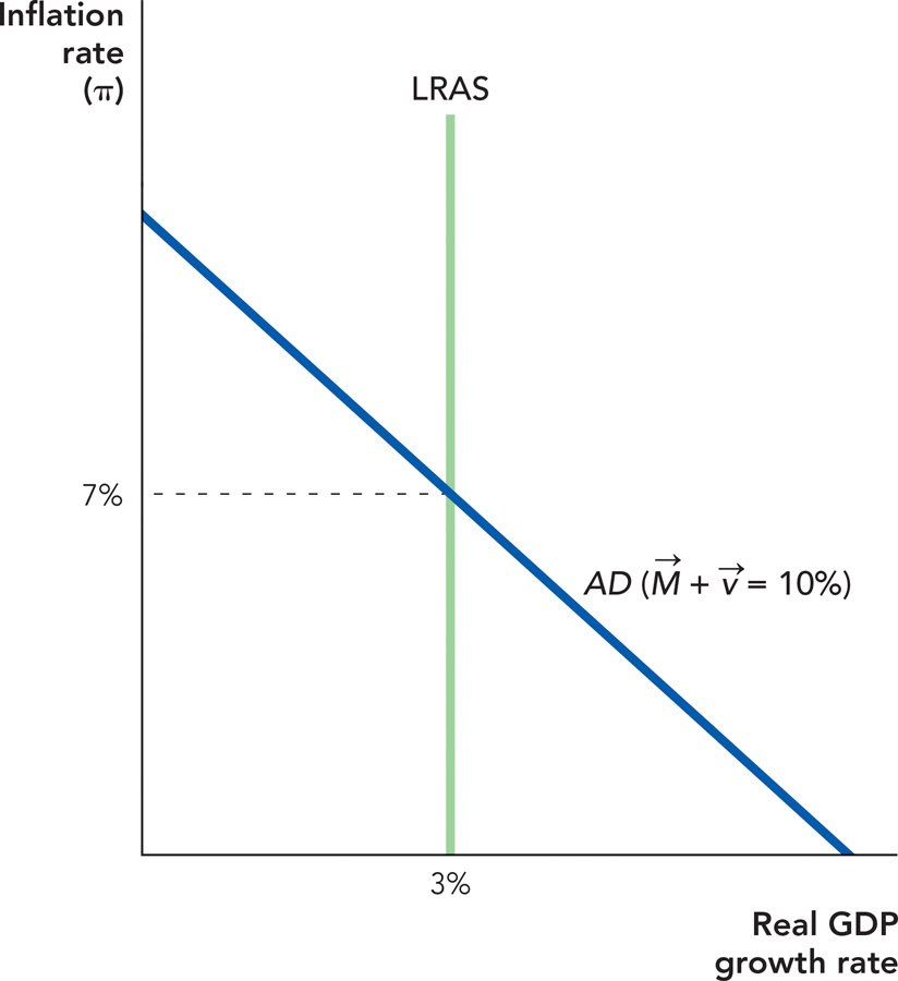
Let’s put the AD and Long-Run Aggregate Supply curve together. This will let us explain how business fluctuations can be caused by real shocks, a way of thinking about business fluctuations often called the “real business cycle” (RBC) model. Figure 13.6 shows an AD curve in which the growth rate of spending is 10% a year and a long-run aggregate supply (LRAS) curve that has a growth rate of 3%. Since = Inflation + Real growth, and = 10%, and Real growth = 3%, we know that inflation is 7% a year. Thus, in this model, the equilibrium inflation rate and growth rate are determined by the intersection of the AD and LRAS curves.

Take a look again at Figure 13.1, which shows the growth rate of U.S. GDP over time. Although the growth rate has averaged about 3% (at an annual rate) per quarter for many years, it has fluctuated around this average. Why?

One reason that the growth rate fluctuates is that economies are continually being hit by shocks, which shift the Solow growth rate. As an example, consider an agricultural economy: Good weather can increase crop production—driving the growth rate up—while bad weather can decrease production, thereby driving down the growth rate.

279

We call these shocks real shocks or productivity shocks because they increase or decrease an economy’s fundamental ability to produce goods and services and, thus, they increase or decrease the Solow growth rate.

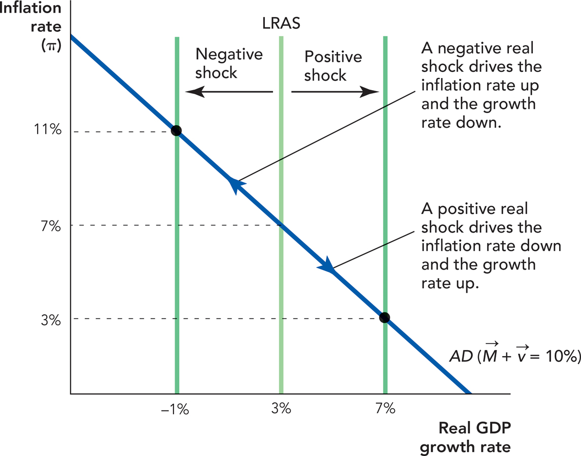
A positive real shock shown in Figure 13.7 shifts the LRAS curve to the right, increasing real growth. The increase in the supply of goods brought about by a higher real growth rate reduces the inflation rate. During the late 1990s, for example, the Internet revolution, a positive real shock, increased the growth rate of the economy. Faster, more powerful computers at lower prices helped to keep inflation low.

A negative real shock shifts the LRAS curve to the left, decreasing real growth. The slower growth rate means fewer new goods to spend money on so the inflation rate increases. In the 1970s, for example, a negative real shock—a sudden, sharp decrease in the relative supply of oil leading to several big jumps in the price of oil—reduced the growth rate and increased inflation.

Shocks to the LRAS curve will change the growth rate and the inflation rate temporarily because the LRAS curve is always shifting back and forth as new shocks hit the economy. Remember from Figure 13.1 that growth is not smooth. Thus, growth rates fluctuate from quarter to quarter, as positive shocks increase growth temporarily and negative shocks reduce growth temporarily. In the United States, growth has fluctuated around approximately 3% for about a century. In different times and places, the average Solow growth rate could be higher or lower depending on growth in the fundamentals—capital, labor, ideas, and institutions—but every economy will always be subject to real shocks so growth will always fluctuate.

280

This way of looking at booms and recessions—the real business cycle (RBC) model or perspective—is a natural extension of the Solow growth model. In the RBC framework, business fluctuations are simply changes in economic growth in the short run driven by real shocks.