Aggregate Demand Shocks and the Short-Run Aggregate Supply Curve
An aggregate demand shock is a rapid and unexpected shift in the AD curve (spending).
Aggregate demand shocks are another type of shock that can hit the economy. An aggregate demand shock is a rapid and unexpected shift in the aggregate demand curve. Since the AD curve is all about spending, we can also say that an aggregate demand shock is a rapid and unexpected shift in spending. To explain why AD shocks matter, we need to introduce the short-run aggregate supply (SRAS) curve and explain the importance of “sticky” (not perfectly flexible) wages and prices.
Before we introduce the SRAS curve, however, let’s give some intuition about where we are going. It takes time for an aggregate demand shock to work its way through the economy. Recall the inflation parable from Chapter 12. In that parable, the government of Zimbabwe prints more money to pay its soldiers. The soldiers use the new money to buy more goods such as bread—that’s an increase in spending, a positive shock to aggregate demand. At first, the baker is delighted when soldiers walk through her door with cash for bread. To satisfy her new customers, the baker works extra hours and bakes more bread. “How wonderful,” she thinks, “with the increase in the demand for bread I will be able to buy more clothes and cabinets.” The baker is expecting to buy clothes and cabinets at the same prices as she paid before the soldiers started to buy more bread. Only later does the baker realize that the soldiers have been buying more of everything, pushing up prices throughout the economy so that her money buys her less than it did before. Once the baker comes to expect rising prices throughout the economy, she raises the price of bread and goes back to producing at the old output level.
The parable tells us that a positive shock to spending increases output at first, but in the long run only increases prices. We know from our basic equation  = Inflation + Real growth that an increase in spending
  must either increase the inflation rate π or the real growth rate. But we also know that in the long run, the real growth rate will be equal to the Solow rate, which is not influenced by the inflation rate, so in the long run an increase in spending will increase the inflation rate alone. The parable, however, tells us that the inflation rate does not necessarily increase immediately in direct proportion to an increase in spending. In the short run, an increase in spending will be split between increases in inflation and increases in real growth—that is the essence of the short-run aggregate supply curve to which we now turn.
The short-run aggregate supply (SRAS) curve is upward-sloping, like that shown in Figure 13.11. An upward-sloping SRAS means that in the short run an increase in aggregate demand will increase both the inflation rate and the growth rate, and a decrease in demand will decrease both the inflation rate and the growth rate.
FIGURE 13.11
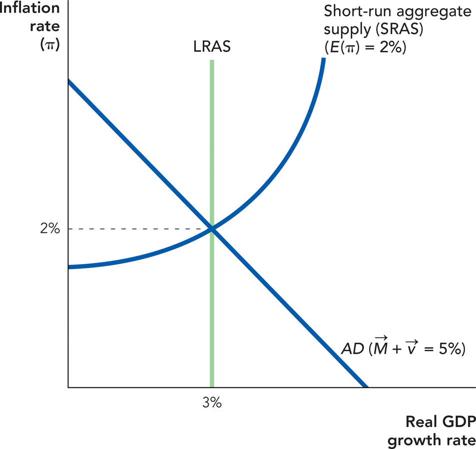
The short-run aggregate supply curve (SRAS) shows the positive relationship between the inflation rate and real growth during the period when prices and wages are sticky.
The rate of inflation that workers and producers expect is written E(π).
Figure 13.12 illustrates the same ideas from the parable but now using the AD, SRAS, and LRAS curves. We start from a position of long-run equilibrium, which means that the inflation rate consumers and firms are expecting must be equal to the actual inflation rate and that the real growth rate must be at the Solow level. Thus, in Figure 13.12, the initial equilibrium is at point a where the real growth rate is at the Solow rate (3%), the inflation rate is 2%, and the expected inflation rate is 2%. Economists often use the symbol π for inflation and E(π) for the expected inflation rate. As we will show shortly, each SRAS curve is associated with a particular rate of expected inflation, so the initial SRAS curve is labeled with E(π) = 2%.
FIGURE 13.12
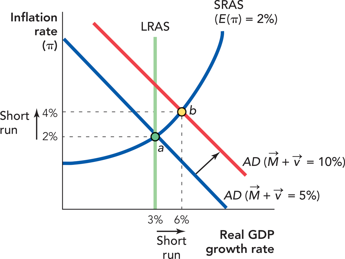
 Shifts the AD Curve Out An increase in AD increases real growth in the short run. The equilibrium moves from point a to the short-run equilibrium at point b.
Now suppose that the growth rate of the money supply increases unexpectedly from 5% to 10%. The injection of more money into the economy increases AD, which, in turn, creates a temporary boom at point b. At b the economy is growing at a 6% rate of real growth with inflation of 4%. Notice that  has increased by 5 percentage points. Some of that increase in spending is reflected in the inflation rate, which increases by 2 percentage points, but some of the increase in spending is reflected in real growth, which increases by 3 percentage points. In the short run, an increase in spending growth is split between increases in inflation and increases in real growth.
Nominal wage confusion occurs when workers respond to their nominal wage instead of to their real wage, that is, when workers respond to the wage number on their paychecks rather than to what their wage can buy in goods and services (the wage after correcting for inflation).
To further explain how a spending increase can create a temporary increase in growth, let’s return to our baker but now imagine that she owns a large bakery. An increase in spending encourages the baker to expand so she offers her workers more overtime opportunities at a higher wage. At first the workers are pleased since they see that their nominal wage—the number on their paychecks—has increased. But as the workers spend their money, they discover that prices elsewhere in the economy are rising so much that even with the overtime, their wages are buying fewer goods and services than before—more work for less real pay! Although the workers’ nominal wages have increased, their real wages—namely the amount of goods and services they can buy with that wage—have decreased. The workers’ eagerness to work harder is what economists call a nominal wage confusion. Eventually, the workers will come to expect the higher inflation rate and they will demand even higher wages to catch up to the higher inflation rate, but in the short run an increase in spending can cause an increase in output.
Menu costs are the costs of changing prices.
Prices also don’t move instantly to their new long-run equilibrium because it is costly to change prices. Economists call the costs of changing prices menu costs because an obvious example is the costs of printing new menus when a restaurant changes its prices. Catalog companies like Lands’ End and L.L. Bean face similar costs for their mail order business. Menu costs also include the costs of upsetting customers with frequent price changes. Menu costs mean that businesses don’t like to change prices every day or even every quarter, so price changes take time.
Firms may also not be sure whether a change in market conditions is temporary or permanent. If firms are unsure, they will hold off on changing prices, at least for a while. Imagine that the price of eggs increases. Does the restaurant change the price of an omelette? If the restaurant knew the price change was permanent, then it probably would. But maybe the price of eggs will decease tomorrow. If the change in the price of eggs is temporary and the firm prints new menus today, it might also have to print new menus again tomorrow, or perhaps incur the risk that consumers search around for a cheaper breakfast. Better to wait and see before changing the prices and printing the new menus.
Over time, however, firms will begin to realize that the price of eggs isn’t coming back down—the increase in price really was permanent and so firms will adjust their menus. Similarly, as prices rise and workers begin to realize that their real wage hasn’t risen, they will demand higher wages. Since wages are a cost to firms, higher wages will in turn lead to higher prices. Wages and prices will continue to increase until the new long-run equilibrium is achieved.
In Figure 13.13, we show what happens in the long run. In the long run, unexpected inflation always turns into expected inflation and the SRAS curve shifts up and to the left; from Old SRAS (E[π] = 2%) to New SRAS (E[π] = 7%). As expectations and prices adjust, more and more of the increase in M is reflected in the inflation rate and less is reflected in the real growth rate. In the long run, after all transitions are complete, all of the increase in  is reflected in the inflation rate—
 increases by 5 percentage points, the inflation rate increases by 5 percentage points, the growth rate returns to the Solow level, and the actual inflation rate comes to equal the expected inflation rate (7%). Thus, an increase in
  increases real growth in the short run—during the period in which prices and wages are sticky.*
FIGURE 13.13
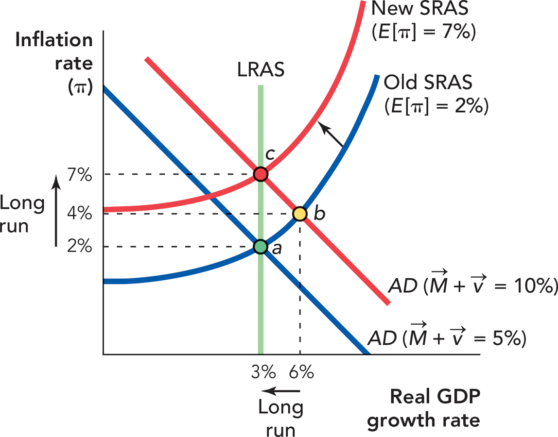
Here is a hint about shifting the SRAS curve. In the long run, people will always come to expect the actual inflation rate (you can’t fool people forever), and in the long run, the inflation rate is found where the LRAS curve intersects the AD curve. In the long-run, the economy must be on the LRAS curve, thus the SRAS curve is always moving toward the point where the LRAS curve intersects the new AD curve (point c in Figure 13.13). Notice that in the new long-run equilibrium, the inflation rate is 7% and the expected inflation rate is 7%. Also, in the long-run equilibrium at point c, growth is equal to the Solow rate—this reflects our intuition that in the long run, money doesn’t influence real growth (money is neutral) but does influence the inflation rate (inflation is a monetary phenomenon).
We also see here a preview of several profound dilemmas in macroeconomic policy. Once we are at the new equilibrium at point c, consumers and producers are expecting an inflation rate of 7%, so to increase the real growth rate above the Solow rate once again, policymakers would have to increase the actual rate of inflation above 7%. Can you see how a policymaker might become trapped in a spiral of ever increasing inflation rates? We will return to this issue in our chapter on monetary policy. Of course, you might ask why not just reduce aggregate demand and return to a lower inflation rate? Unfortunately, prices and wages adjust even more slowly to a fall in AD than to an increase in AD, so a fall in AD can create a severe recession.
Figure 13.14 shows what happens when AD falls due to a fall in  . From an initial equilibrium at point a, the fall in AD shifts the economy to a new short-run equilibrium at point b, creating a small reduction in the inflation rate and a large reduction in real growth. Eventually, the economy will adjust to the fall in
  and it will return to a long-run equilibrium at point c. We don’t show this in detail in Figure 13.14, however, because we want to focus on the recession and why an economy can take a long time to adjust to a decrease in aggregate demand.
FIGURE 13.14
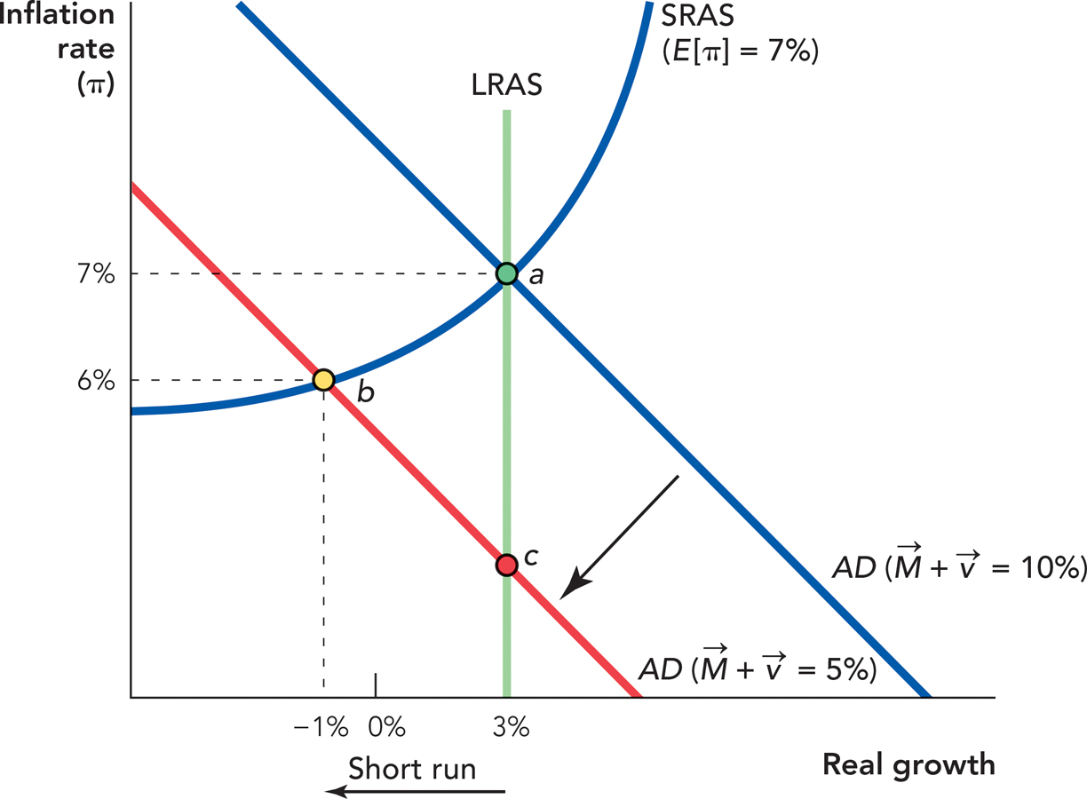
It takes time for a decrease in spending to make its way through the economy for all the reasons that we have already discussed in the case of an increase in spending: namely wages are sticky, menu costs and uncertainty make businesses reluctant to change prices immediately, and expectations take time to adjust. As a result, in the short run, a fall in spending growth is split between a fall in inflation rates and a fall in growth. Most economists, however, believe that prices and wages are especially sticky in the downward direction. Here is one phrase to keep in mind: Prices rise like rockets and fall like feathers.
No one likes to have his or her wages cut or even wage growth reduced, which is one reason that wages are especially sticky in the downward direction. In addition, large union contracts often fix wage growth for several years in advance. So imagine that prices have been going up by 5% and wages by 7% every year for a number of years. Contracts may even have been written guaranteeing wage growth of 7%. Now, however, the inflation rate falls to 2% a year. Workers are expecting wage increases of 7%, but if firms paid that amount, they would be unprofitable. Firms could cut wage growth to 4%, which would give workers the same increase in real wages of 2% that they had before, but how will workers feel when their salary increase is much less than expected? What will happen to morale and motivation? How will a union feel when the company tries to renegotiate its contract? Very often, morale goes down and the union threatens a strike. As a result, firms may find it easier to fire workers or reduce hours than to lower wages. In other words, a fall in aggregate spending will reduce the growth rate.
CHECK YOURSELF
Question 13.5
 The long-run aggregate supply curve is vertical, the short-run aggregate supply curve is not. What explains the difference?
Question 13.6
 Why do inflation expectations form the dividing line between the short run and the long run?
Question 13.7
 Why does a growth in spending lead to an increase in both inflation and real growth in the short run? Why isn’t this the case in the long run?
The economist Truman Bewley interviewed employers and labor leaders, asking them why wages don’t fall during a recession. He concluded that the main reason employers don’t like to cut wages is that if workers see smaller numbers on their paycheck, their morale declines and they often take their anger out on their employers. In contrast, layoffs get the misery out the door. As a result, a fall in aggregate demand can be very dangerous because wages can take a long time to fall, and during that time output declines can be especially large. This is one reason why we have drawn the SRAS curve so it is flatter to the left of the LRAS curve. A decrease in spending that requires expected wage growth to decrease will tend to create a large decrease in the growth rate.
