We know that a firm with market power will price above cost—but how much above cost? Even a firm with no competitors faces a demand curve, so as it raises its price, it will sell fewer units. Higher prices, therefore, are not always better for a seller—raise the price too much and profits will fall. Lower the price and profits can increase. What is the profit-maximizing price?

To maximize profit, a firm should produce until the revenue from an additional sale is equal to the cost of an additional sale. This is the same condition that we discovered in Chapter 11: Produce until marginal revenue equals marginal cost (MR = MC). In Chapter 11, however, calculating marginal revenue was easy because even if a small oil well increases production significantly, the effect on the world price of oil is so small it can be ignored. For a small firm, therefore, the revenue from the sale of an additional unit is the market price (MR = Price). But when a firm’s output of a product is large relative to the entire market’s output of that product (or very close substitutes), a significant increase in the firm’s output will cause the market price of that product to fall. When GSK produces and sells more Combivir, for example, it pushes the price of Combivir down. Thus, for a firm that produces a large share of the market’s total output of a product, the revenue from the sale of an additional unit is less than the current market price (MR < Price).

237

To understand how a firm with market power will price its product, we need to calculate marginal revenue for a firm that is large enough to influence the price of its product.

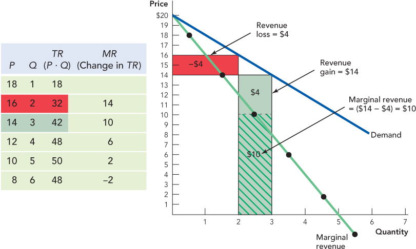
We show how to calculate marginal revenue in the table in the left panel of Figure 13.1. Suppose that at a price of $16 the quantity demanded is 2 units, so that total revenue is $32 (2 × $16). If the monopolist reduces the price to $14, it can sell 3 units for a total revenue of $42 (3 × $14). Marginal revenue, the change in revenue from selling an additional unit, is therefore $10 ($42 – $32). Thus, we can always calculate MR by looking at the change in total revenue when production changes by one unit.

The right panel of Figure 13.1 shows another way of thinking about marginal revenue. When the monopolist lowers its price from $16 to $14, it makes one additional sale, which increases revenues by the price of one unit, $14—the green area. But to make that additional sale, the monopolist had to lower its price by $2, so it loses $2 on each of the two units that it was selling at the higher price for a revenue loss of $4—the red area. Marginal revenue is the revenue gain (green, $14) plus the revenue loss (red, –$4) or $10 (green striped area). Notice that MR ($10) is less than price ($14)—once again, this is because to sell more units, the monopolist must lower the price so there is a loss of revenue on previous sales.

238

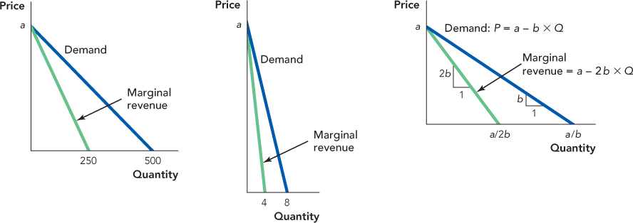
Now that you understand the idea of marginal revenue, here’s a shortcut for finding marginal revenue. If the demand curve is a straight line, then the marginal revenue curve is a straight line that begins at the same point on the vertical axis as the demand curve but with twice the slope.6 Figure 13.2 shows three demand curves and their associated marginal revenue curves. Notice that if the demand curve cuts the horizontal axis at, say, Z, then the marginal revenue curve will always cut the horizontal axis at half that amount, Z/2.

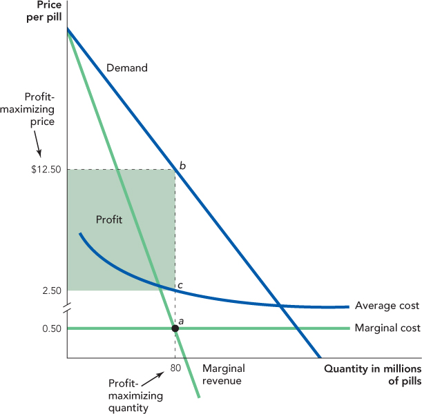
Figure 13.3 sketches the demand, marginal revenue, marginal cost, and average cost curve for a firm with market power, like GlaxoSmithKline. GSK maximizes profit by producing the quantity where MR = MC. In Figure 13.3, this is at point a, a quantity of 80 million units. What is the maximum price at which the monopolist can sell 80 million units? To find the maximum that consumers will pay for 80 million units, remember that we read up from the quantity supplied of 80 million units to the demand curve at point b. Consumers are willing to pay as much as $12.50 per pill when the quantity supplied is 80 million pills, so the profit-maximizing price is $12.50.

We can also use Figure 13.3 to illustrate the monopolist’s profit. Remember from Chapter 11 that profit can be calculated as (P – AC) × Q. At a quantity of 80 million units, the price is $12.50 (point b), the average cost (AC) is $2.50 (point c), and thus profit is ($12.50 – $2.50) × 80 million units or $800 million, as illustrated by the green rectangle. (By the way, the fixed costs of producing a new pharmaceutical are very large so the minimum point of the AC curve occurs far to the right of the diagram.) Recall that a competitive firm earns zero or normal profits but a monopolist uses its market power to earn positive or above-normal profits.

239

Market power for pharmaceuticals can be especially powerful because of the two other effects we mentioned earlier: the “you can’t take it with you” effect and the “other people’s money” effect. If you are dying of disease, what better use of your money do you have than spending it on medicine that might prolong your life? If you can’t take it with you, then you may as well spend your money trying to stick around a bit longer. Consumers with serious diseases, therefore, are relatively insensitive to the price of life-saving pharmaceuticals.

Moreover, if you are willing to spend your money on pharmaceuticals, how do you feel about spending other people’s money? Most patients in the United States have access to public or private health insurance, so pharmaceuticals and other medical treatments are often paid by someone other than the patient. Thus, both the “you can’t take it with you” and the “other people’s money” effects make consumers with serious diseases relatively insensitive to the price of life-saving pharmaceuticals—that is, they will continue to buy in large quantities even when the price increases.

If GlaxoSmithKline knows that consumers will continue to buy Combivir even when it increases the price, how do you think it will respond? Yes, it will increase the price! When consumers are relatively insensitive to the price, what sort of demand curve do we say consumers have? An inelastic demand curve. The “you can’t take it with you” effect and the “other people’s money” effect make the demand curve more inelastic. Thus, we say that the more inelastic the demand curve, the more a monopolist will raise its price above marginal cost.

240

Is it ethically wrong for GSK to raise its price above marginal cost? Perhaps, but keep in mind that in the United States, it costs nearly a billion dollars to research and develop the average new drug. Once we better understand how monopolies price, we will return to the question of what, if anything, should be done about market power.

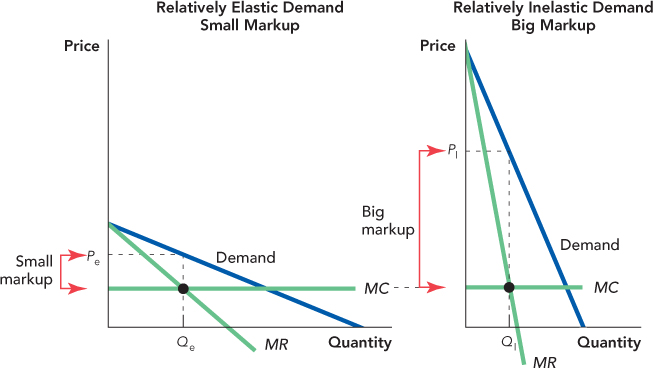
Figure 13.4 illustrates that the more inelastic the demand curve, the more a monopolist will raise its price above marginal cost. On the left side of the figure, the monopolist faces a relatively elastic demand curve, and on the right side a relatively inelastic demand curve. As usual, the monopolist maximizes profit by choosing the quantity at which MR = MC and the highest price that consumers will pay for that quantity. Notice that even though the marginal cost curve is identical in the two panels, the markup of price over marginal cost is much higher when the demand curve is relatively inelastic.

Remember from Chapter 5 that the fewer substitutes that exist for a good, the more inelastic the demand curve. With that in mind, consider the following puzzle. In February of 2014, American Airlines was selling a flight from Washington, D.C., to Dallas for $772. On the same day, it was selling a flight from Washington to San Francisco for $322. That’s a little puzzling. You would expect the shorter flight to have lower costs, and Washington is much closer to Dallas than to San Francisco. The puzzle, however, is even deeper. The flight from Washington to San Francisco stopped in Dallas. In fact, the Washington-to-Dallas leg of the journey was on exactly the same flight!7

Thus, a traveler going from Washington to Dallas was being charged nearly $450 more than a traveler going from Washington to Dallas and then on to San Francisco even though both were flying to Dallas on the same plane. Why?

Here’s a hint. Each of the major airlines flies most of its cross-country traffic into a hub, an airport that serves as a busy “node” in an airline’s network of flights, and most hubs are located near the center of the country. Delta’s hub, for example, is in Atlanta. So if you fly cross-country on Delta, you will probably travel through Atlanta. United’s hub is in Chicago and American Airlines has its hub in Dallas. Have you solved the puzzle yet?

241

Of the flights into the Dallas-Fort Worth airport, 84% are on American Airlines, so if you want to fly from Washington to Dallas at a convenient time, you have few choices of airline. But if you want to fly from Washington to San Francisco, you have many choices. In addition to flying on American Airlines, you can fly Delta, United, or Jet Blue. Since travelers flying from Washington to Dallas have few substitutes, their demand curve is inelastic, like the demand curve in the right panel of Figure 13.4. Since travelers flying from Washington to San Francisco have many substitutes, their demand curve is more elastic, like the one in the left panel of Figure 13.4. As a result, travelers flying from Washington to Dallas (inelastic demand) are charged more than those flying from Washington to San Francisco (elastic demand).

You are probably asking yourself why someone wanting to go from Washington to Dallas doesn’t book the cheaper flight to San Francisco and then exit in Dallas? In fact, clever people try to game the system all the time—but don’t try to do this with a round-trip ticket or the airline will cancel your return flight. As a matter of contract, most airlines prohibit this and similar practices—their profit is at stake!