Let’s put to work what you have learned so far about demand elasticity. Here are two applications.

Using the same inputs of land, labor, and capital, American farmers can produce more than twice as much food today as they could in 1950—that’s an amazing increase in productivity. The increase in productivity means that Americans can produce more food per person today than in 1950. But how much more food can Americans eat? Although it doesn’t always seem this way, Americans want to consume only so much more food even if the price falls by a lot. So what type of demand curve does this suggest? An inelastic demand curve; and remember, when the demand curve is inelastic, a fall in price means a fall in revenues.

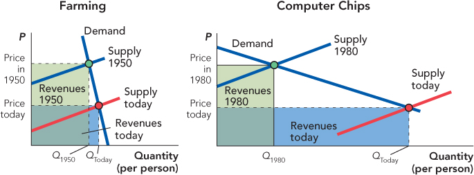
The left panel of Figure 5.4 shows how American farmers have worked themselves out of a job. Increases in farming productivity have reduced cost, shifting the supply curve down and reducing the price of food. But because the demand curve for food is inelastic, the quantity of food demanded has increased by a smaller percentage than the price has fallen. As a result, farming revenues have declined. Notice that in the left panel of Figure 5.4, the blue rectangle (farm revenues today) is smaller than the green rectangle (revenues in 1950)—just as we showed in Figure 5.3.

75

Increases in productivity, however, do not always mean that revenue falls. In the last several decades, productivity has increased in computer chips even faster than in farming. But as the price of computer chips has fallen, the quantity of computer chips demanded has increased even more. Computer chips are now not just in computers but in phones, televisions, automobiles, and toys. As a result, revenues for the computer chip industry have increased and made computing a larger share of the American economy. What type of demand curve does this suggest? An elastic demand curve. The right panel in Figure 5.4 illustrates how an increase in productivity in computing has shifted the supply curve down and reduced prices, but the quantity of computer chips demanded has increased by an even greater percentage than the price has fallen. As a result, computer chip revenues have increased.

The lesson is that whether a demand curve is elastic or inelastic has a tremendous influence on how an industry evolves over time. If you want to be in on a growing industry, it helps to know the elasticity of demand.

It’s hard to defeat an enemy that grows stronger the more you strike against him or her. (See the movies Rocky I, II, III, IV, V, and VI.) The war on drugs is like that. We illustrate with a simple model.

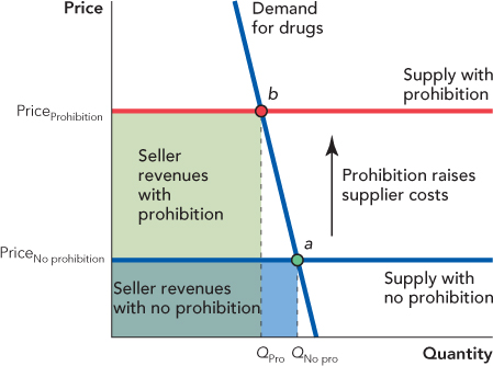
The U.S. government spends over $50 billion a year arresting over 1.5 million people and deterring the supply of drugs with police, prisons, and border patrols.* This, in turn, increases the cost of smuggling and dealing drugs. (The war on drugs also increases the costs of buying drugs. We could include this factor in our model, but to keep the model simple, we will focus on increases in the costs of supplying drugs.) When costs go up, suppliers require a higher price to supply any given quantity so the supply curve shifts up—in Figure 5.5 from “Supply with no prohibition” to “Supply with prohibition.”†

The most important assumption in Figure 5.5 is that the demand curve is inelastic. It’s hard to get good data on how the quantity of drugs demanded varies with the price, but most studies suggest that the demand for illegal drugs is quite inelastic, approximately 0.5. Inelastic demand is also plausible from what we know intuitively about how much people are willing to pay for drugs even when the price rises. Economists have much better data on the elasticity of demand for cigarettes, which one can think of as the elasticity of demand for the drug nicotine and it too is about 0.5.3

76

What happens to seller revenues when the demand curve is inelastic and the price rises? (Review Figure 5.3 if you don’t know immediately.) When the demand curve is inelastic, an increase in price increases seller revenues. In Figure 5.5, the blue rectangle is seller revenues at the no prohibition price; the much larger green rectangle is seller revenues with prohibition. Prohibition increases the cost of selling drugs, which raises the price, but at a higher price, revenues from drug selling are greater even if the quantity sold is somewhat smaller.

The more effective prohibition is at raising costs, the greater are drug industry revenues. So, more effective prohibition means that drug sellers have more money to buy guns, pay bribes, fund the dealers, and even research and develop new technologies in drug delivery (like crack cocaine). It’s hard to beat an enemy that gets stronger the more you strike against him or her.

The war on drugs is difficult to win, but that doesn’t necessarily mean that it’s not worth fighting. Nobel Prize-winning economist Gary S. Becker, however, suggests a change in tactics. Suppose drugs were legal but taxed, much as alcohol is today. Becker suggests that the tax could be set so that it raised seller costs exactly as much as did prohibition (in Figure 5.5 simply relabel “Supply with prohibition” as “Supply with tax”). Since the tax raises costs by the same amount, the quantity of drugs sold would be the same under the tax as under prohibition. The only difference would be that instead of increasing seller revenues, a tax would increase government revenues (by the green rectangle not including the overlap with the blue rectangle). Many of the unfortunate spillovers of the war on drugs—things like gangs, guns, and corruption—could be greatly reduced under a “legal but taxed” system.*

We may be moving toward this type of system in the United States, at least for marijuana. Although marijuana remains illegal under federal law, Colorado and Washington state legalized marijuana for personal use in 2013. So far, the federal laws are not being enforced in those states. In Colorado, legal sales began in 2014, and sales and other taxes are expected to raise around $100 million in revenues annually. The costs of enforcing prohibition will also fall, both for taxpayers and for marijuana sellers and users. The price of marijuana in Colorado appears to be about the same or a bit higher than in states where marijuana remains illegal, which suggests that use will not increase greatly. It is too early to be certain however, whether this experiment in ending prohibition will be fully successful.

Let’s turn now to the elasticity of supply.