3.3 Quantitative Data Descriptions: Median and Quartiles
We began Section 3.2 by looking once again at the top-grossing film data, and asking two questions. First, how much, on average, did a top-grossing film earn, and second, whether the running time for The Lord of the Rings: The Return of the King was unusually long. We answered the first question using the mean; on average, a top-grossing film earned $405 million in the United States. We now turn to numerical descriptive measures that will help us answer the second question.
3.3.1 Locating the Center: Median
Finding the average, or mean, of a data set is one way to locate the center of the distribution of values. The median, the middle value when the data are arranged in size order, is another measure of the distribution’s center. If the number of measurements is odd, there is exactly one measurement in the middle; the median is this measurement. If the number of measurements is even, there are two measurements in the middle, and the median is the mean (average) of these two measurements.
Consider once again the precipitation in San Francisco (data shown below).
| Month | Feb. 2001 | Sept. 2002 | Aug. 2003 | Oct. 2004 | March 2006 | Feb. 2007 | Feb. 2009 | Jan. 2010 | July 2012 | April 2013 |
|---|---|---|---|---|---|---|---|---|---|---|
| Inches | 7.73 | 0.01 | 0.06 | 2.63 | 8.74 | 4.79 | 7.92 | 6.66 | 0.01 | 1.01 |
Arranging the values from smallest to largest we have
0.01, 0.01, 0.06, 1.01, 2.63, 4.79, 6.66, 7.73, 7.92, 8.74.
If we attempt to locate the middle number here, we see that there is not a single value in the middle, but rather, the two values 2.63 and 4.79. The median is then the mean of these two values or 3.71 inches.
The pth-percentile is a number such that p% of the measurements fall at or below that number. So the median is always the 50th percentile since 50% of the measurements fall below that number. In the precipitation data, the number 6.66 is the 70th percentile since 70% of the measurements fall at or below 6.66.
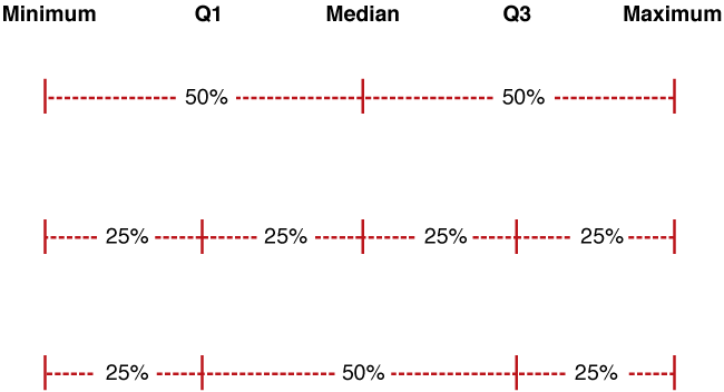
When we use the median as the measure of center, we use quartiles to describe the variability of the data. The median divides the data into its lower 50% and its upper 50%. We call the median of the lower 50% of the data Q1 and the median of the upper 50% of the data Q3. (What happened to Q2? Q2 is actually the median.) Q1, the median, and Q3 divide the set of data values into fourths, or quartiles. Therefore Q1 is the 25th percentile and Q3 is the 75th percentile. Along with the minimum and maximum values, Q1, the median, and Q3 constitute the five-number summary.
When we look at the five-number summary graphically, as indicated in Figure 3.23, we can see various ways to describe how much variability is in the data set:
Here is the five-number summary for the precipitation data.
- Minimum: 0.01
- Q1: 0.06
- Median: 3.71
- Q3: 7.73
- Maximum: 8.74
The interquartile range (IQR) is the distance between Q1 and Q3, namely Q3 – Q1. In this example the IQR is 7.73 - 0.06 = 7.67. The IQR represents the spread of the middle 50% of the data.
So we can conclude that
- 50% of the monthly precipitation totals in our sample were less than 3.71 inches, while 50% were more than 3.71 inches;
- 25% of the monthly precipitation totals in our sample were less than 0.06 inches, while another 25% were more than 7.73 inches.
- the middle 50% of the monthly precipitation totals in our sample were between 0.06 inches and 7.73 inches.
Now Try This 3.22
Use statistical software to find the five-number summary for the running times of the 25 top-grossing films. Between what two values does the middle 50% of running times lie?

The middle 50% of running times lie between and .
Incorrect. When CrunchIt! reports the statistics for Running Time, the values include sample size n, sample mean, and sample standard deviation s, in addition to the five-number summary values we want. Thus, the middle 50% of running times lie between 121 and 153 minutes.
Correct. When CrunchIt! reports the statistics for Running Time, the values include sample size n, sample mean, and sample standard deviation s, in addition to the five-number summary values we want. Thus, the middle 50% of running times lie between 121 and 153 minutes.
3.3.2 Outliers
Let’s return now to the question we asked earlier—was the running time for The Lord of the Rings: The Return of the King unusually long? When we looked at histograms and stem plots, we attempted to identify outliers, data values that were unusual compared to the rest of the data. We looked for gaps at the left-hand or right-hand side in these graphical displays, and tried to judge whether these gaps were significant enough to make us question any data values lying beyond those points. Now we are ready to establish a numerical criterion by which we can determine outliers, and we will illustrate the procedure using the running times of the 25 top-grossing movies.
The procedure statisticians have agreed upon to find outliers is:
- Calculate the interquartile range (IQR), which is Q3 – Q1.
- Multiply the IQR by 1.5.
- Calculate the lower fence, which is Q1 – 1.5*IQR.
- Calculate the upper fence, which is Q3 + 1.5*IQR.
- Outliers are any data values that lie outside the fences; that is, below the lower fence or above the upper fence.
Using the five-number summary from Try This 3.20, and following these steps, we find the fences for the running time data for the 25 top-grossing movies.
- IQR = Q3 – Q1 = 153 – 121 = 32.
- IQR * 1.5 = 1.5 * 32 = 48.
- Lower fence = Q1 – 1.5*IQR = 121 – 48 = 73.
- Upper fence = Q3 + 1.5*IQR = 153 + 48 = 201.
Figure 3.24 shows these values on a number line—the lower fence lies 48 units below Q1, while the upper fence is 48 units above Q3.
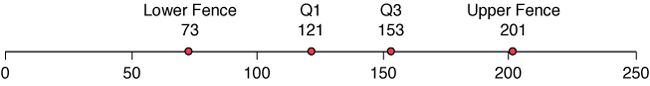
Since the minimum running time of 89 minutes is not outside the lower fence, there are no low outliers. The data value 201 lies on the upper fence. Our criterion for identifying an outlier says that a value must be outside the fences, so the running time of 201 minutes just misses being a high outlier. This example makes clear how the criterion works. Having a strict rule allows us to agree on outliers, rather than having to take differences in opinion into account.
Hence, we see that the 201-minute running time for The Lord of the Rings: The Return of the King, while quite long and unusual compared to the rest of these films, is not an outlier. On a revenue-per-running-minute basis, Shrek 2, which had a running time of 93 minutes and earned $436 million was a better bargain than The Lord of the Rings: The Return of the King, which generated $377 million dollars. However, fans of The Lord of the Rings trilogy might argue that The Return of the King had more artistic merit, as evidenced by its earning 11 Academy Awards, as compared to none for Shrek 2.
Why do we care about outliers? Often, they are interesting just because they are different. A person who is 7 feet tall is much more likely to be noticed than one who is 6 feet tall. Like such a person, an outlier “stands out” from the crowd. If we are sure that the data values are correct (as in the movie running times), an outlier is a curiosity that may help or hinder the point we are trying to make. (Just for the record, it is not valid to remove an outlier from the data just because we don’t like what it does to our results.)
On the other hand, outliers sometimes occur as the result of data collection or data entry errors. If it can be determined that an outlier is the result of such an error, the error should be noted, and the value eliminated from statistical calculations. In a statistics class, the instructor collected student height data, asking for the value in inches. One student reported a height of “6.” Since no one in the class was only 6 inches tall, the error was pointed out, and that value was not used in analyzing the data set. While we might guess that the student was actually 6 feet tall, we cannot assume that this was the mistake and substitute the equivalent 72 inches. The best we can do is to explain why we have chosen to ignore the value in our calculations.
3.3.3 Box Plots
A handy way to display the information from the five-number summary is in a box plot (sometimes called a box-and-whisker plot). A box plot consists of two parts:
- a rectangle (the “box”) whose left-hand edge occurs at Q1 and right-hand edge occurs at Q3, with the median indicated by a vertical line at the appropriate value, and
- two line segments (the “whiskers”), one extending from the left-hand edge of the box to the minimum value and the other extending from the right-hand edge of the box to the maximum value.
Does this sound confusing? Take a look at the following whiteboard video, Box Plots, to see an example.
A look at the box plot for the running times of the movies (in Figure 3.25) will assure you that it is a graph of the five-number summary.
When we draw box plots by hand, we generally draw them horizontally because we are used to looking at number lines in this way. However, a box plot can be drawn vertically as well, and some software packages, including CrunchIt! do so.
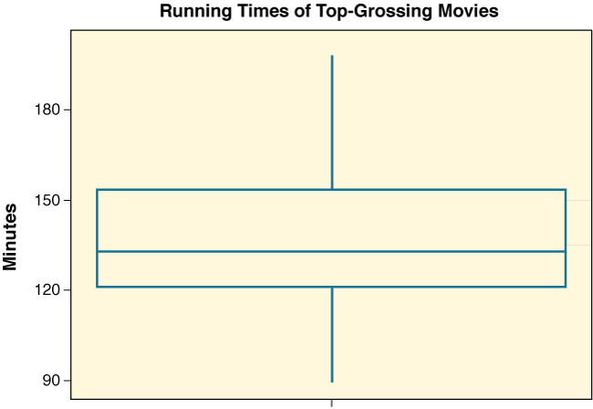
We can see here that the plot indicates that the median lies a little bit above 130, with Q1 close to 120, and Q3 around 150. The whiskers extend to about 90 on the bottom and 200 on the top. This indeed corresponds to the five-number summary we found previously: minimum 89, Q1 121, median 133, Q3 153, and maximum 201.
Recall that we used the information from the five-number summary to determine outliers. Most statistical software allows us to use the fences to determine outliers, and to identify them as separate points beyond the whiskers. This type of box plot is sometimes called a modified box plot. CrunchIt! displays modified box plots. In order to illustrate how a modified box plot appears, we changed the running time of The Lord of the Rings: The Return of the King to 202 minutes to make it an outlier. In Figure 3.26 we see the CrunchIt! plot for this modified data set, showing the outlier as a single point above the end of the whisker. This clearly shows that had The Lord of the Rings: The Return of the King been just one minute longer, its running time would indeed have been an outlier.
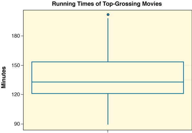
While different software packages display box plots in different ways, they all show the same “box,” which indicates where the middle 50% of the data lie. For the movie data, the middle 50% of the running times lie between 121 and 153. While these values (Q1 and Q3) are not labeled on the graph, we can see that the bottom and top of the box are at these values, respectively.
Now Try This 3.23
Use a modified box plot to determine whether there are any outliers in the January 2010-December 2013 monthly gas price data. Verify your result using the 1.5*IQR criterion.
- According to the box plot there outliers.
- Using the descriptive statistics calculated by CrunchIt!, the IQR is .
- The lower fence is .
- The minimum value is the lower fence.
- The upper fence is .
- The maximum value is the upper fence.
The video StatClips: Exploratory Pictures for Quantitative Data provides examples and comparisons of numerical and graphical measures to describe quantitative data. Note that the video refers to "location" rather than "center."
3.3.4 Mean or Median?
How do we decide which measure of center is more appropriate for a given data set? Let’s consider a couple of examples.
Figure 3.27 shows the distribution of normal body temperatures for 134 individuals, as both a histogram and a box plot.
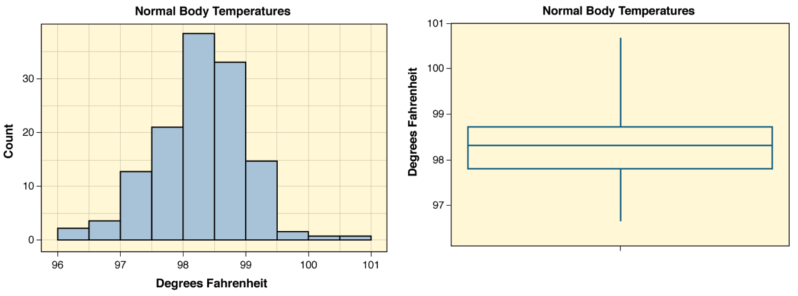
We notice that the distribution is very symmetric; the mean for this data set is 98.55, and its median is 98.60. In this situation, you would probably agree that it does not matter whether we use the mean or the median to measure the center of the distribution.
Table 3.15, below, gives the total compensation in millions of dollars for a simple random sample of heads of America’s 500 biggest companies.
| 31.825 | 3.203 | 6.301 | 1.750 | 21.903 | 19.706 | 6.979 | 1.046 | 3.234 | 1.158 |
| 9.458 | 1.882 | 11.007 | 1.200 | 1.996 | 4.810 | 10.312 | 6.504 | 3.946 | 5.944 |
Figure 3.28 shows a histogram and a box plot of these data. In this case, we see that the distribution is skewed to the right, with an upper outlier.
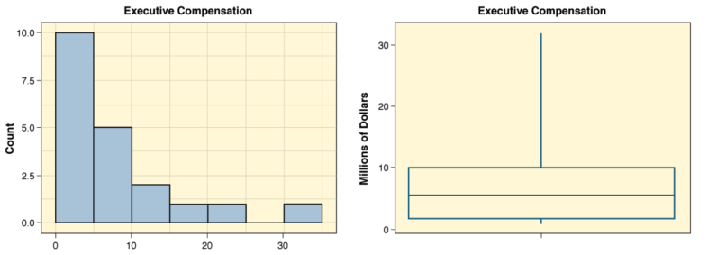
When we calculate the mean and the median, we find that the mean (7.708 million dollars) is quite a bit larger than the median (5.377 million dollars). Which value better represents the center of the distribution? The three largest values (including the outlier) are much larger than the rest, and they cause the mean to be larger than a “typical” measurement. In fact, the mean is larger than 14 of the 20 measurements—not exactly what you would think of as the “center.” So we conclude that here the median is the better measure of the center.
Income distributions, like the one for the sample of executive compensations, are frequently right-skewed. The NPR Story The Income of the “Average American” looks at the relationship between mean and median incomes.
(We will refer students to the LaunchPad's discussion forums to discuss.)
For a skewed distribution such as this, we say that the mean is “pulled away” from the median in the direction of the skewness. So here, the mean is to the right of—that is, larger than—the median. In a left-skewed distribution, the mean is influenced by low values (whether or not they are outliers), and thus is pulled to the left of the median.
When a distribution is symmetric, the mean is a good measure of the center. When we use the mean to measure the center, we typically use the standard deviation to measure the variability. We recall that the standard deviation, which measures variability by considering deviations from the mean, is also affected by extreme values. So like the mean, it is not very useful when the data are skewed. For a skewed distribution, the median is the preferred measure of the center, and we then use the quartiles to measure variability.
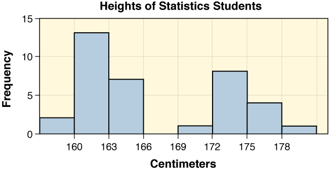
One additional measure of center that is sometimes used is the mode, the measurement (or measurements) that occurs most frequently. A distribution can have one or more modes; however, if all data values occur the same number of times, we say that the distribution has no mode. Recall that we referred to the mode in Section 3.1 when we were describing the shape of histograms. We called a distribution bimodal if its graph had two non-adjacent tall peaks (of roughly equal height), . Bimodal distributions occur more frequently than you might think. A histogram showing the distribution of heights for a class of students (like Figure 3.29) might well be bimodal, with one peak reflecting a common height of females, and the second indicating a common height of males.
Reporting the center and the variability of a set of numerical data gives important information about a distribution. Before choosing a particular combination of measure of center and variability, it is useful to graph the data set, using a histogram, a stem and leaf plot, or a box plot.
If the distribution is symmetric, we typically choose the mean to measure center, and the standard deviation to measure variability. If the distribution is not symmetric, the median is the preferred measure of center, with quartiles used to measure variability.
We also use quartiles in the procedure for determining outliers. Outliers can occur because of natural variation in data, or as a result of data collection or entry errors. When it is possible to characterize an outlier as a genuine error, it can be removed from the data set prior to any numerical analysis. However, such removal (and the reason for it) must be noted.
While it may seem that we concentrate on numerical techniques as we proceed with statistical analysis, it is important to remember that graphs can help us select the numerical measures and techniques that are most appropriate for a particular data set.