5.2 Probability from a Sample Space
We began our discussion of probability with the experiment of tossing a coin, because it provided us with a very simple situation—two equally likely outcomes, Heads and Tails. This experiment allowed us to look at exact, or theoretical probability, and to contrast it with empirical probability and subjective probability. In this section, we will look at further examples of theoretical probability and develop additional rules for probability.
5.2.1 Sample Spaces and Probability
When we perform a probability experiment, the set of all possible outcomes is called the sample space, frequently designated as S. Some sample spaces are very small. When we toss a coin once, the sample space is S = {heads, tails}. Some sample spaces are quite large. If we chose 2 people at random from a class of 30 students, the sample space would include all pairs of students and have over 400 outcomes, all of them equally likely.
For examples like those just described, calculating theoretical probability depends on our ability to list all the outcomes of the sample space and on these outcomes being equally likely. Any experiment with two equally likely outcomes is the same as tossing a coin—the outcomes just have different names. And we certainly don’t want to attempt to write down a sample space with 400 outcomes. So let’s look at some experiments with more than two outcomes but considerably less than 400.
Suppose that we put five pieces of paper in a hat, two red pieces, numbered 1 and 2, and three blue pieces, numbered 1, 2 and 3. If we choose a piece of paper at random, we will get one of a certain color and with a particular number written on it. What is the sample space for this experiment? If we indicate color with the first letter of the color name and give the number written on the paper, then the possible outcomes of the experiment are R1, R2, B1, B2, and B3. Because we define the sample space as the set of outcomes, the sample space would be S = {R1, R2, B1, B2, B3}.
Recall that we defined an event as a collection of one or more outcomes. For this experiment, “getting a blue piece of paper” is an event, as is “getting a piece of paper with the number 1 on it.” What are the probabilities of each of these events?
Before we determine the probabilities, let’s introduce some standard probability notation, which is fairly simple. We use this notation to avoid writing a lot of English, or to clarify matters when we are talking about several similar things. We generally assign events names that are capital letters or numbers (where appropriate). We use the notation P( ) to indicate the probability of whatever event appears inside the parentheses.
So, letting B stand for “getting a blue piece of paper,” and 1 stand for “getting a piece of paper with the number 1 on it,” we want to find P(B) and P(1). Keep in mind that all of the outcomes in this sample space are equally likely. There are five pieces of paper, and three of them are blue, so P(B) = ⅗. Similarly, of the five pieces of paper, two have 1’s on them, so P(1) = ⅖.
How did we calculate these values? In general, the probability of any event E is given by
P(E)=numberofsuccessfuloutcomestotalnumberofoutcomes, provided that the outcomes are equally likely.
By "successful outcomes," we mean those outcomes in which E (whatever it is) occurs. So if event B is "getting a blue piece of paper," only those outcomes in which a blue piece of paper is selected are successful ones.
Now Try This 5.2
Use the sample space S = {R1, R2, B1, B2, B3} to find the probability of each event, and write the answers using probability notation.
The event R = "getting a red piece of paper."
The event 3 = "getting a piece of paper with the number 3 on it."
In the last section, we promised (or threatened, depending on your perspective) to present our basic rules of probability in a more algebraic form—which means in notation. The following table displays the original English versions and their corresponding forms in notation. The two forms are saying the same thing, and you are free to remember whichever one seems easier to you.
| 1. The probability of each event is a number between 0 and 1, inclusive. | 0≤P(E)≤1 |
| 2. The sum of the probabilities for all possible outcomes of the event is 1. | P(S) = 1, where S is the sample space. |
| 3. The probability that an event does not occur is 1 minus the probability that it does occur. | P(not E) = 1 - P(E) |
5.2.2 Examining Probabilities for a Single Event
Let’s consider picking a single card at random from a standard deck of cards. A standard deck of cards has 52 cards, divided into 4 suits of 13 cards each. The suits are called Clubs, Diamonds, Hearts and Spades. Clubs and Spades are black; Diamonds and Hearts are red. Each suit has cards numbered from 2 through 10, a Jack, a Queen, a King, and an Ace. We don’t want to write down the sample space of all 52 cards, so we will just picture it mentally.
Consider the events R = getting a red card, H = getting a Heart, and Q = getting a Queen. What are P(R), P(H), P(Q), and P(not Q)? Each of the 52 outcomes is equally likely; 26 of the outcomes are red cards, so P(R) = 26/52 = ½. Since 13 of the cards are Hearts, P(H) = 13/52 = ¼. There are four Queens in the deck, so P(Q) = 4/32 = 1/13 and P(not Q) = 1- 1/13 = 12/13.
Finally, we will look at one more experiment before we move on to more complicated events. We want to examine the probabilities associated with having a boy in a three-child family. For each child, determining the sex is the same as tossing a coin—each outcome, male or female, is equally likely. (We make this assumption so that we can use theoretical probability here. If we used empirical probability, based on actual birth records, we would find that slightly more than 50% of newborns are boys, and thus slightly less than 50% are girls.)
An easy way for us to determine the sample space for this experiment, without missing any of the possibilities, is to make a tree diagram. A tree diagram displays branches, each of which represent a possible outcome for a trial of the experiment. Because this example involves a three-child family, the tree is three branches deep. To find the sample space, we have to follow every possible path to the end of the tree. In Figure 5.1 we let B = having a boy, and G = having a girl and consider the possible outcomes.
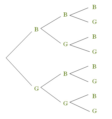
If you have only one child, there are only two possibilities. If you have two children, there are now four—two choices for the first child, and whatever that outcome, plus two choices for the second make four possible arrangements altogether. Similarly, each of the four possible arrangements of sex for the first two children has two choices for the third, so there are eight possible outcomes for this experiment.
If we follow each branch to the end of the diagram, we get the outcomes BBB, BBG, BGB, BGG, GBB, GBG, GGB, and GGG. The sample space for this experiment is then S = {BBB, BBG, BGB, BGG, GBB, GBG, GGB, GGG}, where, for example, BGB indicates that the first child is a boy, the second is a girl, and the third is the boy.
What is the probability of having two boys in a three-child family? Here we run into a bit of difficulty between what we say in English and what we mean in statistics. When we say “having two boys” do we mean only two boys or does the outcome with three boys count here as well? (If a family has three boys, then it certainly has two!) We will clarify this question by being a bit more explicit. Let’s consider the following three questions.
- What is the probability of exactly two boys in a three-child family?
- What is the probability of at least two boys in a three-child family?
- What is the probability of at most two boys in a three-child family?
The first question, about exactly two boys in a three-child family is pretty straightforward. Three of the eight equally likely outcomes (BBG, BGB, GBB) have exactly two boys, so the desired probability is ⅜.
The second and the third question require us to distinguish between “at least” and “at most.” Some students have trouble with this distinction—until they think about money. If you have at least $5 in your pocket, you have $5 or more; if you have at most $5 in your pocket, you have $5 or less.
So "at least two boys" means two or more boys; in this case, 2 or 3 boys. Now the outcomes we are interested in are BBG, BGB, GBB, and BBB, so the probability is 4/8 = ½. And “at most two boys” means two or less boys; in this case, no boys, 1 boy, or 2 boys. The outcomes satisfying this condition are GGG, BGG, GBG, GGB, BBG, BGB, GBB, so the probability for this event is ⅞. Notice that the only outcome not included in this event is the one in which there are more than two boys, namely BBB.
We define a random variable as a numerical variable whose values result from the outcomes of a random experiment. The number of boys in a three-child family is a random variable, whose possible values are 0, 1, 2, and 3. If we let X represent this random variable, then the probabilities calculated above can be written in notational form as
- P(X=2)=38;
- P(X≥2)=12;
- P(X≤2)=78.
Now Try This 5.3
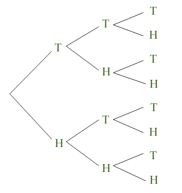
The number of Tails that occur in three tosses of a fair coin is a random variable. If we let Y represent this random variable, use a tree diagram to find each probability. Fill in the blank to complete each probability fraction.
P(Y=1) = /2
P(Y≥1) = /2
P(Y≤1) = /8
5.2.3 Probability for Two or More Events
Continuing with the three-child family example, let’s define event C as “the first child is a girl” and event D as “the third child is a boy." We call these two events independent because the outcome of the first has no effect on the outcome of the second. In this case, knowing the sex of the first child doesn’t give you any information about the sex of the third child.
We know that the probability of each sex for each child is ½, so P(C) = P(D) = ½. What if we want to know about the probability of both events happening, that is, P(C and D)? If we look once again at the sample space S = {BBB, BBG, BGB, BGG, GBB, GBG, GGB, GGG}, we see that the outcomes GBB and GGB are the only two in which the first child is a girl and the third child is a boy. Therefore P(C and D) = 2/8 = ¼.
How does the probability of the events occurring together relate to the probabilities of the events happening separately? A fourth rule of probability tells us that, if two events are independent, the probability that they both occur is the product of their separate probabilities. In notational form,
P(E and F) = P(E)·P(F), as long as E and F are independent.
Thus, the probability that the first child is a girl and the third child is a boy is given by P(C and D) = P(C) • P(D) = ½•½ = ¼, the same value we got when we calculated the probability directly from the sample space. This rule can be extended to any number of events, but it is important to remember that it applies only when the events are independent. For this reason, the rule is frequently referred to as the Multiplication Rule for Independent Events.
Finally, one more question about our three-child family—what is the probability that the first child is a girl or the third child is a boy? Here we use the mathematical definition of “or,” which is “one or the other or both.” So we are looking for outcomes in which the first child is a girl, the third child is a boy, or both. Again examining the sample space, we see the outcomes GBB, GBG, GGB, and GGG represent the first child being a girl. The outcomes BBB, BGB, GBB. and GGB represent the third child being a boy. If we count all these successful outcomes as listed, we would be counting GBB and GGB twice—once as “first child girl” and once as “third child boy.” We want to count each successful outcome only once, so the number of unique outcomes in the list is 6. Thus, P(C or D) = 6/8 = ¾.
That leads us to our final probability rule: the probability that one event or another occurs is the sum of their separate probabilities minus the probability that both events occur. That is,
P(E or F) = P(E) + P(F) - P(E and F).
A special case of this rule applies if the two events have no outcomes in common. The events are then called disjoint, and P(E and F) = 0. There is no need, however, to remember an additional rule, because this one works all the time, regardless of whether the events are disjoint.
Now Try This 5.4
The graphic below shows all the possible outcomes when two dice are rolled. Find each probability from the sample space and fill in the blank to complete each probability fraction. Then, where appropriate, verify your answer by using the probability rules.
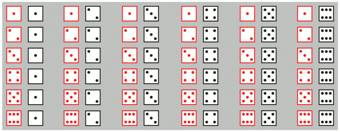
- Event A = first die shows a "two."
- Event B = the second die shows a "five."
- Event C = the sum of the numbers on the dice is even.
(a) P(A and B) = /36
(b) P(A or B) = /36
(c) P(B and C) = /12
(d) P(B or C) = /12
(a) From the sample space, P(A and B) = 1/36. Because A and B are independent, P(A and B) = P(A) • P(B). P(A) = 6/36 = ⅙, and P(B) = 6/36 = ⅙, so P(A and B) = 1/36.
(b) From the sample space, P(A or B) = 11/36. P(A or B) = P(A) + P(B) – P(A and B) = 6/36 + 6/36 - 1/36 = 11/36.
(c) From the sample space, P(B and C) = 3/36 = 1/12. Because A and B are not independent, the multiplication rule for independent events cannot be used.
(d)From the sample space, P(B or C) = 21/36 = 7/12. P(B or C) = P(B) + P(C) – P(B and C) = 6/36 + 18/36 - 3/36 = 21/36 = 7/12.
Another example of an interesting probability problem is one that’s known as the “birthday problem.” Let’s say that there are thirty students in your statistics class. What do you think is the probability that at least two of you share the same birthday? Is it small, perhaps less than 20%, moderate, around 50%, or high, greater than 80%? Take a minute to think about what your intuition tells you and then listen to a short discussion of this problem.
When most people are introduced to this problem they think at first that there is a low chance of finding a match, but it turns out that the answer is much larger than most people think. With 30 people in a room, there are 435 different ways to pair two people, so there are lots of potential matches!
The solution is not hard to find if we use the P(not E) = 1 – P(E) rule. Rather than finding the probability that at least two people share a birthday, we’ll answer the opposite question, that is, we’ll compute the probability that no two people share the same birthday and subtract this from one.
If there are just two people present, then there is a 364/365 = 99.7% chance that they do not have the same birthday, because there are 364 of 365 possible days that the second person’s birthday can fall on so that it doesn’t match the first person’s birthday. If a third person joins these two, there is a 363/365 × 364/365 = 99.2% chance that this person’s birthday is different from the other two. Likewise, if a fourth person joins the group, there is a 362/365 × 363/365 × 364/365 = 98.4% chance that none of the four share the same birthday.
If we stick to this strategy, we’ll see that there is a 29.4% chance that no one in a group of 30 has the same birthday. This means that there is a 1 - .294 = .706 or 70.6% chance that at least two people share the same birthday! Are you surprised that this probability is so high? Maybe equally surprising to you is that you only need 23 people in a room for there to be a 50% chance that there will be at least one pair of people with the same birthday!
Another counter-intuitive situation is discussed in the previous video clip. Suppose that I tell you that a family has two children and one is a boy. What is the probability that the other child is a boy? The Math Guy says that it is ⅓, but that most people think the correct answer is actually ½. Let’s see why this is so. Because we’re told that (at least) one child is a boy, the sample space for this scenario is S={BG, GB, BB}. Each of these three outcomes is equally likely, and the event “the other child is a boy” is only satisfied by the outcome “BB.” Therefore the probability is in fact ⅓.
If all this probability seems difficult to you, don’t be alarmed. Some probability questions (like those about poker hands in Section 5.1) are very difficult. And, as we pointed out, intuition often fails us. Our goal in this section is for you to explore the basic ideas and rules of probability in settings where you can determine the sample space. A bit of practice with these concepts will probably make things clearer for you.
A good way to approach the exercises is to proceed as in the “at least one boy” example above—find the answers directly from the sample space, and then verify your answers using the rules when they apply.