8.2 Hypothesis Tests for a Population Proportion
A typical National Hockey League goalie saves around 90% of shots on goal. As a recreational hockey player, your friend claims to be able to perform as well as a professional. You doubt this claim, and challenge him to prove it. You attend his next game, at which he saves 26 shots out of 30. On the basis of this performance, do you reject his claim or not?
The purpose of hypothesis testing is to use statistical methods to evaluate competing claims. An example that demonstrates the idea behind hypothesis testing (without any actual statistics) involves the competing claims to the invention of the ice cream sundae by two different cities. Listen to the story The Great Ice Cream Sundae Debate to hear about the evidence in favor of each city. According to the high school students who undertook the study, which city's claim is supported by the evidence?
Since the claim refers to his long term performance, you shouldn’t expect him to save exactly 90% of shots, 27 in this case, each and every game. But you are evaluating the claim based on this one particular game. If his claim is true, he ought to save about 90% of shots almost all the time. But what do we mean by “about?” If he saved all 30 shots on goal, you would be likely to accept his claim. If he saved only 15 shots, you would probably disagree (even if he argues that he merely had a bad day). Somewhere between 15 and 30, you will give him the benefit of the doubt, but where is that point? Is the 26 shots he saved enough? What about 25 or 24?
Deciding whether sample evidence is strong enough to reject a claim about one or more population parameters (like the percentage of shots on goal saved) is at the heart of the statistical tests we study in the next several chapters.
8.2.1 Sampling Distribution of ˆp Revisited

Photo Credit: scyther5/Shutterstock
According to an analysis of 17 studies involving over 5000 patients, the use of a nicotine patch was effective in achieving a 6-month abstinence from tobacco smoking in 22% of those treated. A group of researchers theorized that a combination therapy of nicotine inhaler plus nicotine patch might be more effective than use of the patch alone. In a double-blind, randomized, placebo-controlled trial, one group of 200 patients received the nicotine inhaler plus nicotine patch for 6 weeks, then inhaler plus placebo patch for 6 weeks, then inhaler alone for 14 weeks. At the end of 6 months, 50 (25%) of these patients were completely abstinent from smoking. Do these data provide evidence to conclude that the combination therapy is more effective for smoking cessation than the patch alone?
In order to conclude that the combination therapy is better, we would expect to see a percentage of abstinent patients higher than 22%. But how much higher? We know that samples vary, and so do their proportions. The 25% cessation rate in this sample might seem a lot better, but is it high enough? We want to make a decision based on statistical principles, not on our intuition. (It turns out, that people’s intuition in such matters is not very good). We want to see results that are statistically significant, that is, unlikely to have occurred merely by chance.
To evaluate the evidence, we must understand how a sample statistic would vary if the new treatment were no better than the old. We need to examine the variability of the sample proportion of abstinent subjects in all samples of size 200 if the combination treatment produces only a 22% cessation rate.
As we discussed in Section 8.1, as long as the sample size is large enough (and it is), the sample proportions will be approximately normally distributed, with μˆp=p and σˆp=√p(1−p)n. In this situation, then, the sample proportions of abstinent subjects will have a normal distribution with μˆp=0.22 and σˆp=√0.22(1−0.22)200≈0.03. Based on the Empirical Rule, we would expect that 68% of sample proportions of abstinent subjects would lie between 0.19 and 0.25, and 95% would be between 0.16 and 0.28, even if the combination therapy produces the same result as the patch alone. Having 50 of 200 (25%) patients abstinent from smoking cannot be considered all that unusual.
To determine just how unusual this result is, we can employ our normal probability techniques. Since the sampling distribution of ˆp has a mean of 0.22 and standard deviation 0.03, we determine that P(ˆp≥0.25)=0.1587, as shown in the figure below.
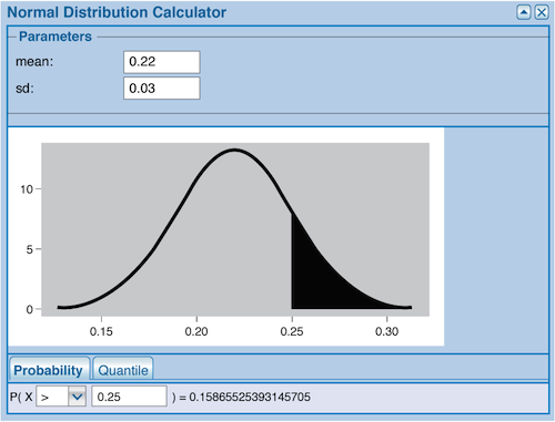
This means that if the combined therapy were no better than the patch alone, we would expect to see a sample proportion of 0.25 or higher nearly 16% of the time. These results could very easily have occurred merely by chance—when the population proportion is 0.22, a sample proportion at least this high occurs roughly 16% of the time as a result of variation in the random samples selected.
This probability calculation is central to our decision making. We are interested in rejecting established claims only when results from the sample are unusual, that is, more extreme than that expected due to sampling variability.
Now Try This 8.7
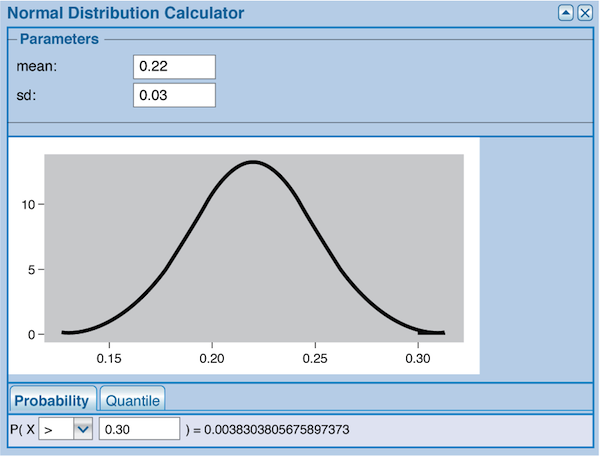
Suppose that the researchers conducted a second study using the same methods and found that 30% of 200 subjects were abstinent from smoking after 6 months. Find P(ˆp≥0.30) to determine how likely sample results like these would be if the combination therapy were no better than the patch alone. Round your answer to four decimal places.

P(ˆp≥0.30)= .
Correct.
Using the same sampling distribution model as before (normal, with μˆp=0.22 and σˆp=0.03), P(ˆp≥0.30)=0.0038. Since these results are unlikely (occurring merely by chance less than 4 times out of 1000), a sample proportion this large would be very good evidence that the combination therapy is better than the patch alone.
Incorrect.
Using the same sampling distribution model as before (normal, with μˆp=0.22 and σˆp=0.03), P(ˆp≥0.30)=0.0038. Since these results are unlikely (occurring merely by chance less than 4 times out of 1000), a sample proportion this large would be very good evidence that the combination therapy is better than the patch alone.

8.2.2 The Process of Hypothesis Testing

Photo Credit: Kostas Tsipos/Shutterstock
Now that we have considered an example of evaluating the evidence against a particular claim, let’s use the example to formalize the process of hypothesis testing. Throughout the rest of the course, each hypothesis test we perform will consist of 5 parts:
- Null hypothesis
- Alternative hypothesis
- Test statistic
- Results
- Conclusion
The basic premise of hypothesis testing is that we are trying to promote one claim by contradicting another. We begin a test of a hypothesis by stating the claim we want to contradict. For the time being, this claim is a statement about the value of a population proportion. (In later chapters, we will test claims about different parameters, as well as about relationships between variables.) We call this statement the null hypothesis, and indicate it using the symbol H0, which we read as “H-naught,” with “naught” being a British term for zero. H0 is often referred to as the hypothesis of no difference.
In this example, H0 is the statement that the proportion of abstinent subjects using the combination therapy is the same as that using the patch alone. That is, H0 is p=0.22. The value in the null hypothesis can come from previous research (as it did here), or from a statement made by an individual or a company (“3 out of 4 of the students who take our prep course increase their SAT scores by 160 points.”)
Next, we present the alternative claim or alternative hypothesis, which we call Ha (“H-a”), with the a indicating “alternative.” This is the claim that we will support if evidence from the sample makes it unlikely that H0 is true. For the smoking cessation treatment, Ha is the statement p>0.22.
If it seems to you that we are going about this in a backwards fashion, we are. We start by asserting that what we want to disprove (H0) is actually true, and we evaluate our sample evidence based on this assumption. Oddly enough, it is frequently easier to show that something is false than that its opposite is true.
The way that we will contradict the null hypothesis is by calculating a test statistic, a number we use to decide just how unusual our sample results are. In this case, since the sampling distribution for the sample proportion is approximately normally distributed, we find the z-score for our particular sample proportion. This will tell us how far (in standard deviation units), and in what direction, our sample proportion is away from the mean of the sampling distribution.
Recalling that, in general, z=measurement−meanstandarddeviation, we find that z0.25=0.25−0.220.03=1. This means that a sample proportion of 0.25 lies 1 standard deviation to the right of the mean, μˆp=0.22, of the sampling distribution.
Our results consist of a statement of how unusual our sample results are, given in terms of the P-value of the test. The P-value is the probability, given that the null hypothesis is true, that we would obtain a test statistic this extreme or more so, merely by chance. Since z-scores are values in a standard normal distribution, the P-value represents the probability that the z-score falls into a particular tail of the standard normal curve (or far enough out on either tail).
How do we decide between one or two tails? Our alternative hypothesis tells us the direction(s) that we are interested in.
- If we hope to show that the population proportion is larger than the hypothesized value in H0, then we consider how likely it is that the test statistic would fall at least as far in the right tail as it did, and we perform a right-tailed test. In simple terms, if Ha looks like p > a number, then the test is right-tailed.
- If we hope to show that the population proportion is smaller than the hypothesized value in H0, then we consider how likely it is that the test statistic would fall at least as far in the left tail as it did, and we perform a left-tailed test. So if Ha looks like p < a number, then the test is left-tailed.
- If we want to show that the population proportion is just different from the hypothesized value, then we consider the likelihood that the test statistic would fall as far either to the left or the right as it actually did. Then we perform a two-tailed test. If Ha looks like p ≠ a number, then the test is two-tailed.
For the smoking cessation study, the researchers want to show that the combined therapy does better than the patch alone, so we look at how likely it is that the test statistic would fall at least as far to the right as it did. The normal probability area we calculated for ˆp=0.22 shows that the area of the right tail, and thus the P-value for this test, is 0.1587 (rounded to 4 decimal places). This evidence is insufficient to reject H0.
In the conclusion, we restate our results in terms of the real-world situation. In this case, we find that a test statistic this larger or larger would occur merely by chance nearly 16% of the time if the proportion of those who remained abstinent at 6 months when treated with the combination therapy were 0.22. This result is not unlikely; therefore, we find that the sample evidence is insufficient to conclude that the combination therapy is better than the patch alone.
8.2.3 How to Do a Hypothesis Test about p
In our introduction of hypothesis testing above, we did a lot of defining and explaining that you won’t need to do when you are asked to perform such a test. The procedure below gives five basic steps that you should use to do a hypothesis test about p. Here p0 indicates the specific number (between 0 and 1 since it is a proportion of successes), determined by the particular situation.
- State the null hypothesis.
H0:p=p0 - State the alternative hypothesis based on the claim to be supported. Choose one of the following.
Ha:p<p0 or Ha:p>p0 or Ha:p≠p0 - Report the test statistic.
Test statistic: z = (give value) - Report the P-value.
Results: The P-value is (give value) - State the conclusion in context.
Conclusion: (describe strength of evidence for rejecting the null hypothesis)
Before we use this method in an example, we need to look more closely at some of the details involved. First, the null and alternative hypotheses are statements about a population proportion, p. There is no reason whatsoever for us to test a hypothesis about the sample proportion, ˆp, because we know exactly what the sample proportion is. So H0 and Ha are never written in terms of ˆp. The role of the sample proportion ˆp in this process is to provide the evidence by which we test the hypothesis about the population proportion p.
Second, we need to decide how often we are willing to be wrong. Recall that we faced a similar dilemma with confidence intervals in Section 8.1, and we decided, in general, that being wrong more than 10% of the time was not acceptable. That is the conclusion that we will draw again here—the usual line in the sand that statisticians are unwilling to cross. If the P-value is larger than 0.10, we will say that the evidence is insufficient to reject the null hypothesis. For P-values between 0 and 0.10 (including 0.10), we will use the following adjectives to describe the strength of the evidence:
- 0.05< P-value ≤ 0.10 → moderate
- 0.01< P-value ≤ 0.05 → strong
- P-value ≤ 0.01 → very strong
The graphic below shows (not to scale) the P-values and corresponding adjectives.
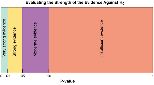
We matched these adjectives with the specific intervals of P-values so that you will have a consistent way to translate the P-value into English. Do real statisticians abide by such arbitrary guidelines? Certainly not, but they have years of experience interpreting statistical tests. A researcher conducting a hypothesis test evaluates the P-value in light of the situation involved. If the consequences of rejecting the null hypothesis are serious or costly, he or she requires stronger evidence than if the test involves (say) people’s opinions on a current issue.
Our guidelines, arbitrary though they are, reflect the fact that the smaller the P-value, the stronger the evidence against the null hypothesis (and so in favor of the alternative). So use these adjectives as a beginner’s guide to interpreting the P-value, always remembering that in the real world, the final decision about rejecting the null hypothesis must take into consideration the consequences of doing so.
Although determining the required probability above was not very difficult, we did have to first find the appropriate z-score and then the corresponding standard normal probability. Fortunately, most statistical software will perform hypothesis tests from sample data, reporting both the test statistic and the P-value. We will take advantage of available software to simplify the hypothesis test process.
Please review the whiteboard Hypothesis Test for a claim about p.
8.2.4 Hypothesis Tests Using Technology
Let’s return to the smoking cessation problem and proceed to do the hypothesis test using our 5-step format and statistical software. To summarize the situation: in previous studies the use of a nicotine patch alone was effective in achieving a 6-month abstinence from smoking in 22% of those treated. In a double-blind, randomized, placebo-controlled trial, one group of 200 patients received combination therapy. At the end of 6 months, 50 of these patients were abstinent from smoking. Do these data provide evidence to conclude that the combination therapy is more effective for smoking cessation than the patch alone?
Using CrunchIt! to perform a hypothesis test for this situation, we find the following.
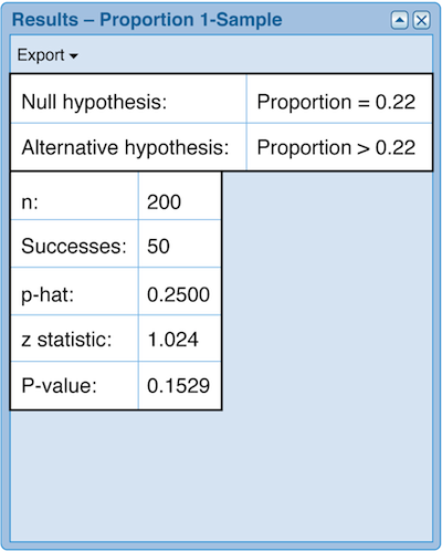
While different software provides the information in slightly different ways, each one should display the null and alternative hypotheses, the sample proportion, the z-statistic and the P-value.
Now for the hypothesis test itself:
H0:p=0.22
Ha:p>0.22
Test statistic: z = 1.024
Results: The P-value is 0.1529.
Conclusion: This sample provides insufficient evidence to conclude that the combination therapy is more effective for smoking cessation than the patch alone.
When we looked at these data earlier, we rounded σˆp to two decimal places to make applying the Empirical Rule easier. The results from CrunchIt! kept more decimal places, and made the z-statistic slightly larger. A larger positive z-statistic cuts off a smaller right-hand tail area and thus a smaller P-value.
We failed to reject the null hypothesis because our P-value was 0.1529. This means that even if the combination therapy were no better than the patch alone, we would get a test statistic as large or larger than 1.024 about 15 times out of every 100 in repeated sampling. If we reject the null hypothesis based on evidence like this, we would be drawing the wrong conclusion about 15 times out of every 100, when we repeated the experiment over and over and over.
It is important to note that failing to reject the null hypothesis is not equivalent to accepting the null hypothesis. The null hypothesis involves one claim about the population proportion, namely that p=0.22. Based on one set of sample data, we found that ˆp=0.25. A 95% confidence interval for p based on this sample proportion is (0.18999, 0.31001). Our hypothesized value of 0.22 is in this interval of reasonable values for the population proportion. But this interval also indicates that it’s plausible that p might be 0.18999, or 0.31001, or any other number between these two. Therefore it is incorrect to accept H0:p=0.22. Instead we conclude that we don’t have enough evidence to support the alternative hypothesis that p>0.22.
The P-value of a two-tailed test is double that of a one-tailed test with the same test statistic. Such a P-value is appropriate because we would decide whether to reject the null hypothesis based on a test statistic this far away from 0 regardless of whether the test statistic were to the left or the right of the 0.
Now Try This 8.8
According to a Monitoring the Future survey, 42.6% of 12th graders in the United States reported having used marijuana at some point in their lifetime. A superintendent believed that this claim is not valid for 12th grade students in her school district. Based on a simple random sample of 105 seniors in her school district, she found that 31 had used marijuana at some point. Complete the hypothesis test to determine whether there is statistical evidence that the percentage of 12th graders in the superintendent’s school district who had used marijuana differed from the national percentage. Round answers to 3 decimal places.

- H0:p =
- H0:p
- Test statistic z =
- Results: P-value =
- Conclusion: These data provide evidence to conclude that the percentage of 12th graders in the superintendent’s school district who had used marijuana differed from the national percentage.
Correct. In order to complete the test using the 5-step format indicated, we first use software to perform the hypothesis test.
- H0:p=0.426
- H0:p≠0.426
- Test statistic z=−2.710
- Results: The P-value is 0.006.
- Conclusion: This sample provides very strong evidence to conclude that the proportion of those seniors in the superintendent’s district that had used marijuana differed from the national percentage of 42.6%.
Incorrect. In order to complete the test using the 5-step format indicated, we first use software to perform the hypothesis test.
- H0:p=0.426
- H0:p≠0.426
- Test statistic z=−2.3147
- Results: The P-value is 0.006.
- Conclusion: This sample provides very strong evidence to conclude that the proportion of those seniors in the superintendent’s district that had used marijuana differed from the national percentage of 42.6%.
8.2.5 Conditions for Hypothesis Tests about p
As we did with confidence intervals, we have explained the process of performing a hypothesis test before considering the conditions needed to do so. The conditions required for a hypothesis test about the population proportion p are very similar to those for a confidence interval for p. In fact, only the fourth condition is different, because we calculate expected numbers of successes and failures based on the hypothesized value of p.
Before conducting a hypothesis test about p you should verify the following:
- The data come from a simple random sample from the population of interest.
- Individual measurements (success or failure) are independent.
- The sample size is no larger than 10% of the size of the population.
- The expected number of successes, np0, is at least 10 and the expected number of failures n(1 - p0) , is at least 10, where p0 is the hypothesized value of p.
If you cannot make a convincing argument that the conditions are satisfied, you should not perform a test that is, in effect, meaningless. As before, we are most concerned about the nature of the sample itself. You should verify that the sample is (at least an approximation of) a simple random sample or the result of a randomized comparative experiment.
Let’s check these conditions for the hypothesis test about the percentage of high school seniors in a certain school district who have tried marijuana.
- The study used a simple random sample of seniors from the school district. This is the most important condition for our appropriate use of inference, and it is satisfied in this case.
- Given that the sample was a simple random sample, individual measurements were independent as long as the students were interviewed or surveyed without consulting each other.
- For the sample size of 105 to represent less than 10% of the population of interest, the school district must have less than 1050 seniors. Unless the school district was small, this is likely to be the case.
- The sample included np0=105∗0.426=44.73 successes, and n(1−p0)=105∗0.574=60.27 failures. Each of these is larger than 10.
We will be considering a number of other hypothesis tests in later chapters. Each test has not only its own conditions, but also its own test statistic. To distinguish between these tests, we generally give them names based on both what is being tested and the test statistic used. For that reason, we refer to this hypothesis test about p as the one proportion z-test or the one sample z-test for a proportion.